The Evolution of FlashAttention
We present a mathematical & technical overview of FlashAttention and its evolution across versions 1 to 4. We explain why IO-aware design became central to scalable transformers and how these kernels shape modern long-context LLMs as memory patterns and hardware limits shift. We then describe the changes across versions with Triton examples and place these kernels in the context of recent work on efficient attention. We close by outlining principles that can guide the next generation of attention algorithms.
Note: For brevity, we’ve omitted code implementations in this post. You can view the source and notebooks on GitHub here.
Introduction
The fundamental concept that underpins the transformer architecture is Attention. This was originally developed as an enhancement to RNNs for machine translation
The importance of this mechanism can be explained with the help of the following example
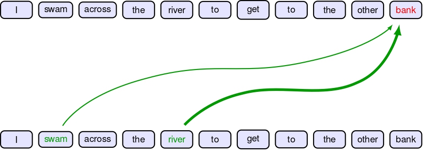
Consider the sentence “I swam across the river to get to the other bank.” The word “bank” has multiple meanings—it could refer to a financial institution or a riverbank. The attention mechanism helps the model understand context by weighing relationships between words. In this case, the model attends strongly to words like “swam,” “across,” and “river,” which provide contextual clues that “bank” refers to a riverbank rather than a financial institution.
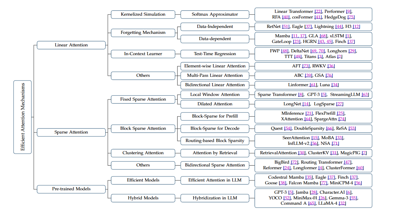
Therefore, the Attention mechanism has become a critical mechanism driving the growth of Large Language Models. Over the years, several variants of the attention mechanism have been proposed such as Multi Query Attention (MQA) (cite), Grouped-Query Attention (GQA), Multi-Head Latent Attention (MLA), etc. For instance, here’s a non-exhaustive taxonomy of efficient attention mechanisms
However, the transformer’s attention mechanism has a limitation: it scales quadratically both in time and memory with sequence length, resulting in $O(n^2 \cdot d_{\text{model}})$ time complexity and $O(n^2)$ memory complexity. For example, a 2,048-token sequence requires 16 MB of memory for the attention matrix; at 16,384 tokens, this increases to 1GB per layer. A mathematical proof is presented in Appendix A. This quadratic scaling makes it prohibitive for processing long sequences beyond 8K-16K tokens without specialized optimizations
The FlashAttention series by Tri Dao
Background
GPU Memory Hierarchy
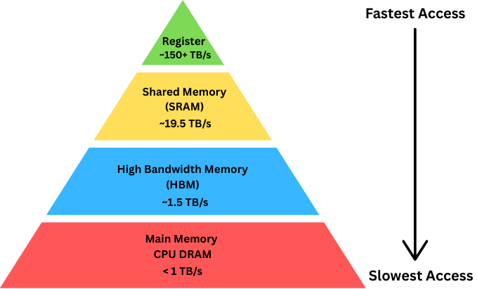
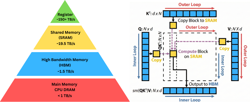
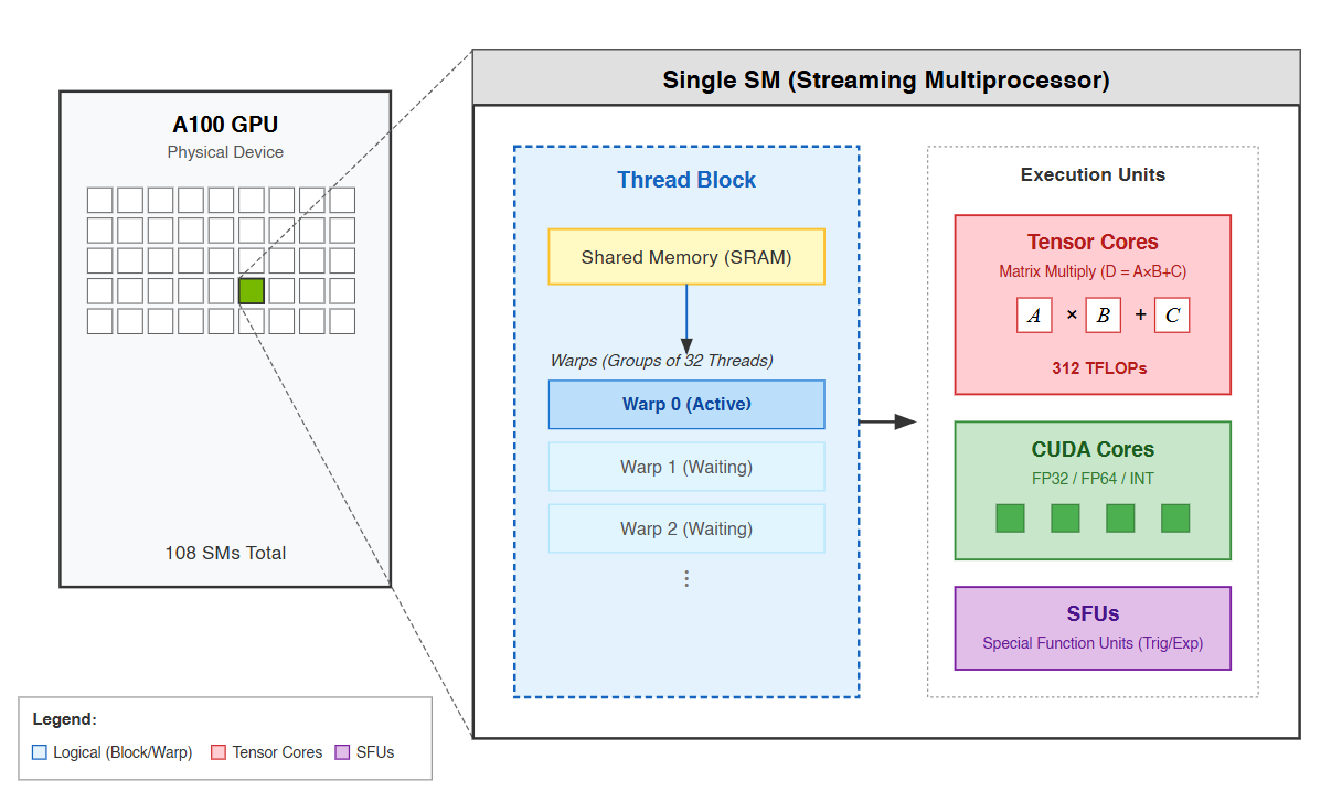
Every modern processor faces the same fundamental challenge: fast storage is expensive and small, while large storage is slow and cheap. Modern GPUs organize memory into a hierarchical form which has five distinct levels, each with different characteristics, different access patterns, and different implications for your code. Starting from the fastest and smallest and working towards the slowest and largest, these levels are: registers, shared memory, L1 cache, L2 cache, and global memory (as shown in the above Figure). At the top of the memory hierarchy sit registers, the fastest storage available on a GPU. Each thread running on the GPU has access to a private set of registers - typically up to 255 registers per thread on modern NVIDIA architectures. These registers feed directly into the computational units. When a thread performs an arithmetic operation, the operands come from registers and the result goes back to registers. There is no separate “register access” operation visible to the programmer; registers are simply where the active data lives. The register file on a single Streaming Multiprocessor contains 65,536 registers with each register holding 32 bits. This gives 256 kilobytes of register storage per SM, and these registers are dynamically shared among all threads running on that SM
Unlike registers, which are private to each individual thread, shared memory (SRAM) is shared among all threads in a thread block. It is the primary mechanism for threads to cooperate and communicate and is explicitly managed by the programmer rather than automatically managed by the compiler. Shared memory provides a staging area for data that multiple threads need to access. Rather than having each thread read the same value from slow global memory, one thread can read it once into shared memory, synchronize with the other threads, and then all threads can read from fast shared memory. Secondly, it enables algorithms that require threads to exchange data. This is used explicitly by FlashAttention.
At the bottom of the hierarchy sits global memory - the large DRAM pool that provides the bulk of a GPU’s storage capacity. An H100 for example, has 80GBs of HBM memory, operating at around 3,000 gigabytes per second of bandwidth. This is where your input data starts, where your output data goes, and where any persistent state lives. It is also by far the slowest level of hierarchy, with individual access latencies reaching 400 to 800 clock cycles depending on architecture and access pattern.
| Memory Level | Capacity | Bandwidth | Latency | Programmer Control |
|---|---|---|---|---|
| Registers | 256 KB/SM | ~100 TB/s | 0 cycles | Automatic |
| SRAM | 192 KB/SM | 19 TB/s | ~20 cycles | Explicit |
| L2 Cache | 40-50 MB | 12 TB/s | ~200 cycles | Transparent |
| HBM | 40-80 GB | 1.5-2 TB/s | ~500 cycles | Explicit |
When we look at the GPU memory hierarchy in detail, we see a sharp difference in both latency and bandwidth across levels. Registers and shared memory sit close to the compute units and respond within a few cycles. HBM sits hundreds of cycles away with higher bandwidth but much higher latency. This separation means that the location of data often dictates runtime. As an example, the A100 GPU has 40GB of high bandwidth memory (HBM2e) with bandwidth 1.6TB/s and 192KB of on-chip SRAM per each of 108 streaming multiprocessors with bandwidth estimated around 19TB/s
Attention is memory bound despite $O(N^{2})$ compute
The efficiency of a kernel is governed by its arithmetic intensity, defined as the number of floating-point operations (FLOPs) performed per byte of memory access. Arithmetic Intensity is commonly used to measure whether operations can be classified as either compute-bound or memory-bound. A process is memory-bound when the execution speed is limited by how fast data can be moved between memory (HBM/RAM) and the processor cores, rather than by how fast the cores can compute. Typical examples include elementwise operations such as activation, dropout and reduction operations such as sum, softmax, batch norm, layer norm. A process is compute-bound when the execution speed is limited by the raw processing power (FLOPS) of the cores such as Matrix Multiplication, Convolution
\[\text{Arithmetic Intensity} = \frac{\text{FLOPs}}{\text{Bytes Accessed}}\]Standard Attention involves three primary stages
- Matrix Multiplication: $ S = Q K^T $
- Softmax: $ P = \text{softmax}(S) $
- Matrix Multiplication: $ O = P V $
The matrix multiplications ($QK^T$ and $PV$) are compute-bound operations with high arithmetic intensity ($O(N^2 d)$ FLOPs vs $O(N^2)$ IO). However, the intermediate Softmax operation is memory-bound. It requires reading the entire $N \times N$ matrix $S$ from HBM, performing reduction operations, and writing the resulting $P$ matrix back to HBM. This $O(N^2)$ memory traffic saturates the HBM bandwidth, leaving the powerful Tensor Cores idle. (Detailed Proof provided in Appendix B)
FlashAttention V1
One of the hardware-efficient mechanisms now widely adopted across different providers is Fast and Memory-Efficient Exact Attention with IO-Awareness, or FlashAttention. The “IO-Awareness” part of the title describes its core technical principle: optimizing data movement between GPU memory hierarchies.
FlashAttention addresses the dual challenges of speed and memory consumption in transformers, especially on long sequences, by rethinking attention algorithms through the lens of GPU memory hierarchy awareness. The key insight is minimizing data movement between high-bandwidth memory (HBM) and on-chip SRAM.
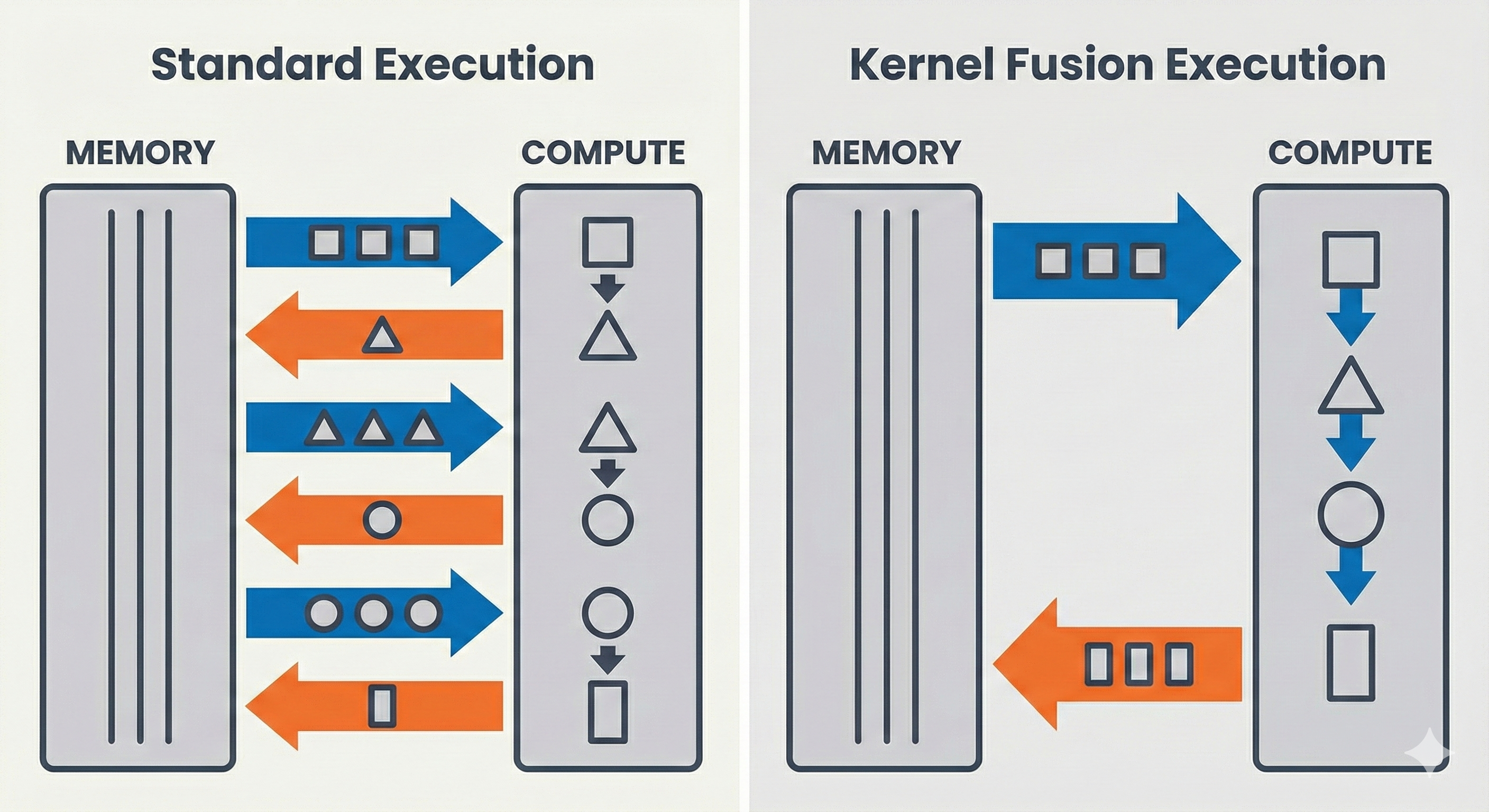
FlashAttention v1, published at Neural Information Processing Systems 2022 by Tri Dao and collaborators, introduced two key innovations: tiled attention that processes blocks of queries, keys, and values entirely in SRAM, and an online softmax algorithm that computes exact softmax incrementally without materializing the full attention matrix.
Online Softmax Algorithm Enables Incremental Computation
Standard softmax computation requires three sequential passes over the data, making it inherently memory-intensive. The first pass finds the maximum value for numerical stability. The second pass computes exponentials and accumulates the normalization sum. The third pass normalizes each element. This three-pass structure can be expressed mathematically as follows:
Given a vector $x \in \mathbb{R}^n$, the numerically stable softmax is computed in three passes:
\[\text{Pass 1:} \quad m = \max_{i} x_i\] \[\text{Pass 2:} \quad d = \sum_{i=1}^{n} e^{\,x_i - m}\] \[\text{Pass 3:} \quad \text{softmax}(x)_i = \frac{e^{\,x_i - m}}{d}\]This approach ensures numerical stability by preventing overflow in the exponential computation. However, this three-pass dependency creates a critical bottleneck: we must materialize the entire attention matrix in HBM before proceeding. The softmax operation requires global information—specifically, the denominator in Pass 2 must sum over all $N$ elements. This seemingly requires loading the full row into memory before computing any output, making the process extremely memory I/O intensive and defeating attempts to tile the computation efficiently.
The breakthrough came from online softmax, an algorithmic technique that computes softmax incrementally in blocks while maintaining running statistics for the maximum and the sum of exponentials. This method was originally discovered by Milakov and Gimelshein
Algebra of Online Softmax
Online softmax allows combining partial results without revisiting the raw data. In a streaming (block-wise) setting, we process the sequence in chunks. Let’s assume we have processed the first block of keys and have a local maximum $m_{old}$ and a local unnormalized sum $\ell_{old}$ (where $\ell = \sum e^{x_j - m}$). Now, we load a new block of keys and compute their raw scores. From this new block, we find a local maximum $m_{block}$ and a local sum $\ell_{block}$.
For each block, we compute local statistics independently. The block size is chosen such that each block fits comfortably in SRAM, allowing us to process it entirely on-chip.
Running maximum (after processing new block):
\[m_{new} = \max(m_{old}, m_{block})\]with initial condition: $m_{old} = -\infty$ for the first block
Running sum (relative to current maximum):
\[\ell_{new} = \sum_{j} e^{x_j - m_{new}}\]with initial condition: $\ell_{old} = 0$ for the first block
Recurrence Relation for the Sum
The mathematical insight is the rescaling formula for $\ell_{new}$. To combine the old and new blocks into a valid global state without accessing the old data, we need to express the new sum in terms of the old statistics.
Starting from the definition:
\[\ell_{new} = \sum_{j \in \text{old}} e^{x_j - m_{new}} + \sum_{j \in \text{block}} e^{x_j - m_{new}}\]Key transformation: Express terms using the old maximum $m_{old}$:
\[e^{x_j - m_{new}} = e^{x_j - m_{old}} \cdot e^{m_{old} - m_{new}}\]Therefore, for the old block terms:
\[\sum_{j \in \text{old}} e^{x_j - m_{new}} = e^{m_{old} - m_{new}} \sum_{j \in \text{old}} e^{x_j - m_{old}} = e^{m_{old} - m_{new}} \cdot \ell_{old}\]Similarly, for the new block terms:
\[\sum_{j \in \text{block}} e^{x_j - m_{new}} = e^{m_{block} - m_{new}} \sum_{j \in \text{block}} e^{x_j - m_{block}} = e^{m_{block} - m_{new}} \cdot \ell_{block}\]Combining both:
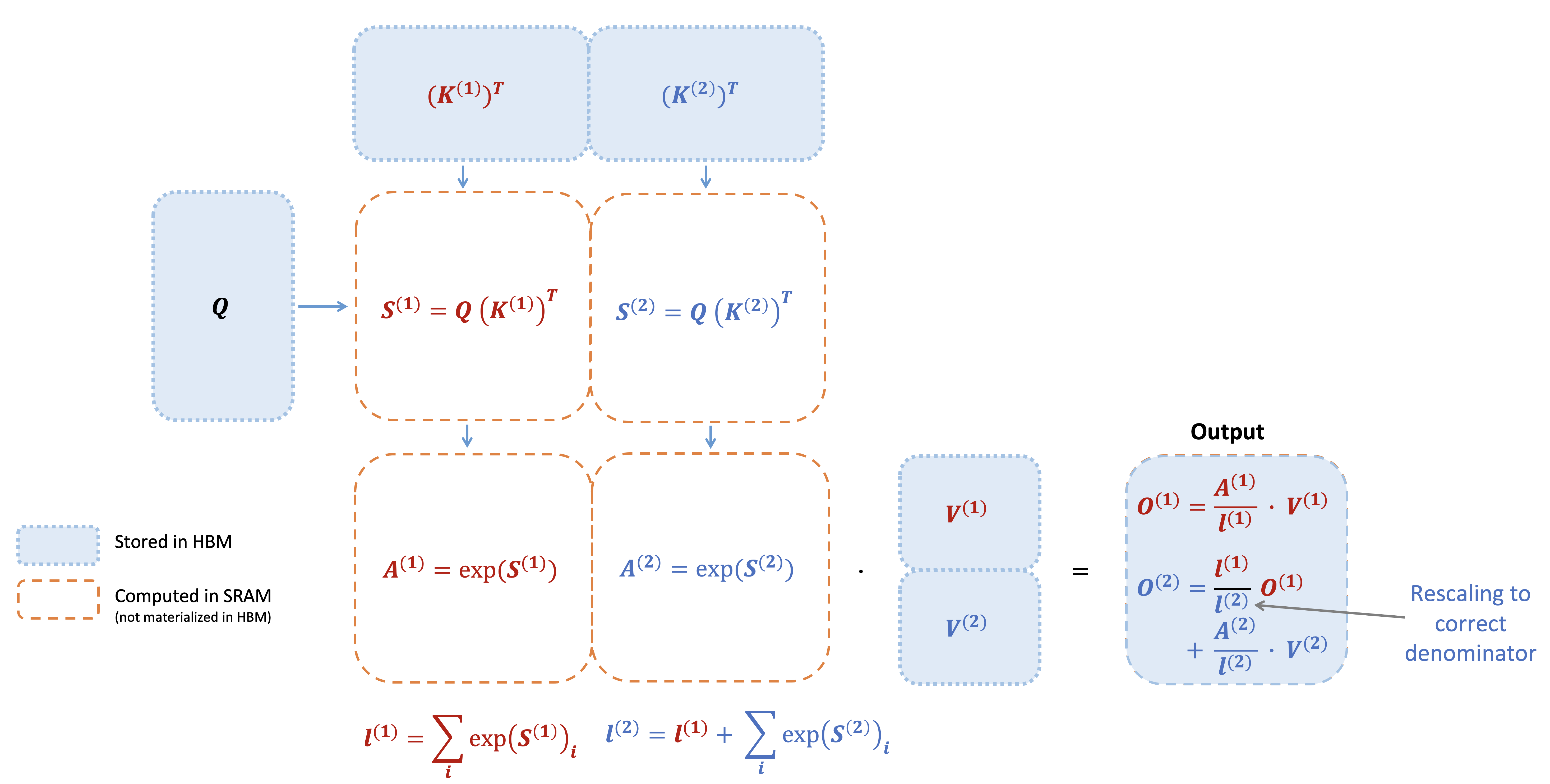
\[\boxed{\ell_{new} = e^{m_{old} - m_{new}} \cdot \ell_{old} + e^{m_{block} - m_{new}} \cdot \ell_{block}}\]We can define the correction factor $\alpha = e^{m_{old} - m_{new}}$. This is the rescaling equation for online softmax. It allows us to update the running sum using only the previous statistics ($m_{old}$ and $\ell_{old}$) and the new block statistics, without ever loading the earlier blocks from HBM again. The exponential correction terms ensure numerical stability throughout the incremental computation by properly rescaling all exponentials relative to the current global maximum. This reduces the operation from 3 passes to 2 passes
Forward Pass
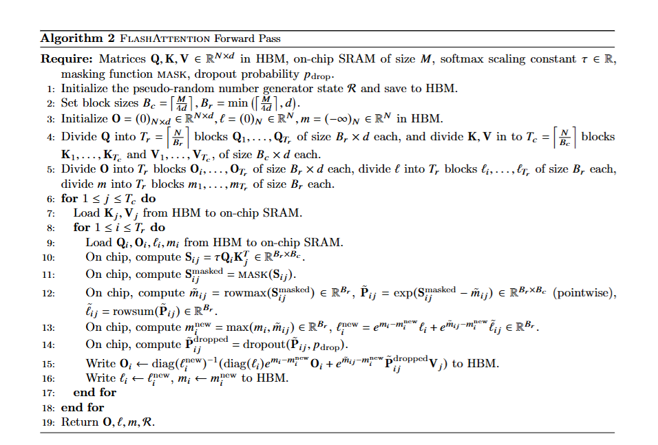
For each attention head, FlashAttention reduces memory reads and writes by tiling. It loads small blocks of queries, keys, and values from GPU HBM into fast on-chip SRAM, computes attention for that block, and updates the output before moving on to the next block. This limits how often data moves between slow and fast memory, which is the main bottleneck on modern GPUs. Cutting this movement often gives a 2–4× speedup in practice.
Mathematical Derivation
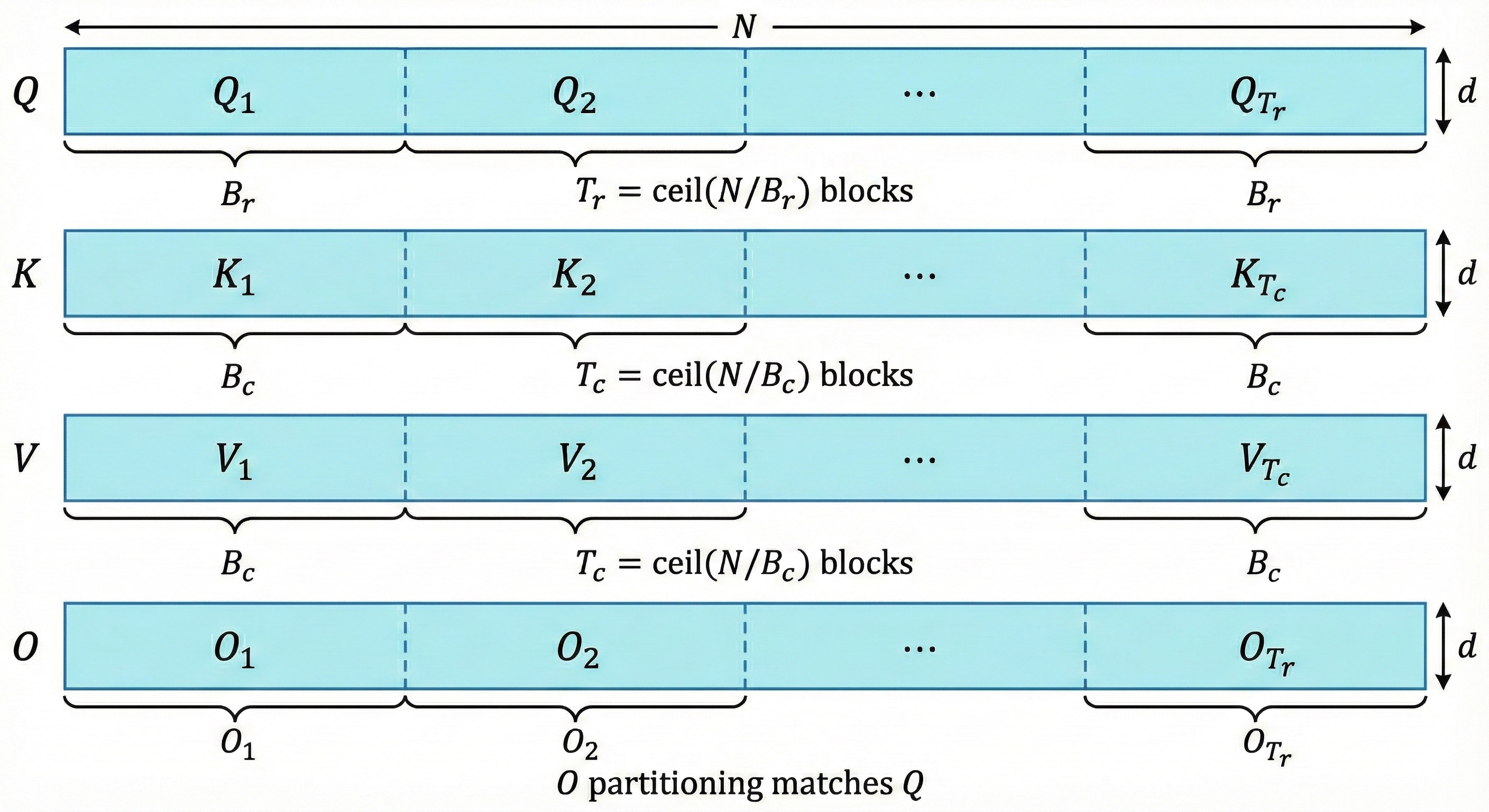
We define the block sizes based on the available SRAM size $M$. Let $B_c$ be the block size for columns (dimension along $N$ for $K, V$), and let $B_r$ be the block size for rows (dimension along $N$ for $Q, O$). The key constraint is $4 B_c d \le M$ to ensure that $K, V$ blocks and various buffers fit in SRAM. Usually, we set $B_c \approx \lceil \frac{M}{4d} \rceil$ and $B_r \approx \min(\lceil \frac{M}{4d} \rceil, d)$.
The matrices are divided into blocks as follows:
- $Q$ is divided into $T_r = \lceil N/B_r \rceil$ blocks: $Q_1, \dots, Q_{T_r}$
- $K$ and $V$ are divided into $T_c = \lceil N/B_c \rceil$ blocks: $K_1, \dots, K_{T_c}$ and $V_1, \dots, V_{T_c}$
- $O$ is divided into $T_r$ blocks: $O_1, \dots, O_{T_r}$
Ideally, to minimize HBM writes of the output $O$, we want to load a block of $Q$, iterate over all blocks of $K, V$, accumulating the result, and then write $O$ once. However, FlashAttention V1 actually uses an outer loop over $K, V$ and an inner loop over $Q$ to better utilize the SRAM for the larger $K, V$ blocks, though conceptually the accumulation happens per query row.
Initialization:
We initialize the output matrix $O = 0 \in \mathbb{R}^{N \times d}$, the running sum vector $\ell = 0 \in \mathbb{R}^N$, and the running maximum vector $m = -\infty \in \mathbb{R}^N$. These statistics will be updated incrementally as we process each block.
Outer Loop (iterating over $K, V$ blocks, $j = 1, \dots, T_c$):
-
Load Key-Value blocks: Load $K_j, V_j \in \mathbb{R}^{B_c \times d}$ from HBM to on-chip SRAM. These blocks remain in SRAM throughout the inner loop.
Inner Loop (iterating over $Q$ blocks, $i = 1, \dots, T_r$):
-
Load Query block and statistics: Load $Q_i \in \mathbb{R}^{B_r \times d}$, $O_i \in \mathbb{R}^{B_r \times d}$, $\ell_i \in \mathbb{R}^{B_r}$, $m_i \in \mathbb{R}^{B_r}$ from HBM to SRAM.
-
Compute attention scores: Compute $S_{ij} = Q_i K_j^\top \in \mathbb{R}^{B_r \times B_c}$. This matrix multiplication is performed entirely in SRAM, computing the raw attention scores between the current query block and key block.
-
Compute local statistics: For the current block, we compute:
\[\tilde{m}_{ij} = \text{rowmax}(S_{ij}) \in \mathbb{R}^{B_r}\](maximum score in each row)
\[\tilde{P}_{ij} = \exp(S_{ij} - \tilde{m}_{ij}) \in \mathbb{R}^{B_r \times B_c}\](pointwise exponential with local normalization)
\[\tilde{\ell}_{ij} = \text{rowsum}(\tilde{P}_{ij}) \in \mathbb{R}^{B_r}\](sum of exponentials in each row)
-
Update running statistics: Using the online softmax rescaling formula:
\[m_i^{\text{new}} = \max(m_i, \tilde{m}_{ij})\](update global maximum)
\[\ell_i^{\text{new}} = e^{m_i - m_i^{\text{new}}} \ell_i + e^{\tilde{m}_{ij} - m_i^{\text{new}}} \tilde{\ell}_{ij}\](rescale and accumulate sum)
-
Update output: We incrementally update the attention output. First, compute partial output contribution:
\[\tilde{V}_{ij} = \tilde{P}_{ij} V_j\](weighted sum of values for current block)
Then combine with running output using the rescaling formula:
\[O_i^{\text{new}} = \text{diag}(\ell_i^{\text{new}})^{-1} \left( \text{diag}(\ell_i) e^{m_i - m_i^{\text{new}}} O_i + e^{\tilde{m}_{ij} - m_i^{\text{new}}} \tilde{V}_{ij} \right)\]This rescales the old output and adds the new contribution, then normalizes by the updated sum.
-
Write back to HBM: Write $O_i^{\text{new}}, \ell_i^{\text{new}}, m_i^{\text{new}}$ back to HBM, updating the global state for this query block.
-
In practice, to avoid numerical instability from dividing by $\ell_i$ at every step, the algorithm often stores the unnormalized output (let’s call it $U_i = O_i \cdot \ell_i$) and only divides by $\ell_i$ at the very end of the computation or maintains the invariant correctly. The formulation above effectively rescales the previous running average to match the new magnitude determined by the new maximum.
Complexity Analysis
The efficiency of FlashAttention is theoretically grounded in its IO complexity. We analyze the number of HBM accesses required by comparing standard attention with FlashAttention.
Standard Attention IO Complexity

For standard attention, the HBM accesses are:
- Read $Q, K, V$: $O(Nd)$
- Write $S = QK^T$: $O(N^2)$
- Read $S$: $O(N^2)$
- Write $P = \text{softmax}(S)$: $O(N^2)$
- Read $P$ and $V$: $O(N^2) + O(Nd)$
- Write $O = PV$: $O(Nd)$
Total: $\Theta(N^2)$ HBM accesses (assuming $N \gg d$)
FlashAttention IO Complexity
FlashAttention’s tiled algorithm significantly reduces memory traffic:
Outer loop (over $K, V$ blocks, $j = 1, \dots, T_c$): Each iteration loads blocks $K_j, V_j$ into SRAM. Since the outer loop iterates over all $K, V$ blocks, these matrices are loaded once in total: $O(Nd)$.
Inner loop (over $Q$ blocks, $i = 1, \dots, T_r$): For each outer iteration, the inner loop loads $Q_i$, $O_i$, $\ell_i$, $m_i$ from HBM.
- Size of $Q_i$: $B_r \times d$
- Total inner loop iterations: $T_c \times T_r$
- Total loading of $Q$: $T_c \times (T_r \times B_r d) = T_c \times Nd$
Since $T_c = \lceil N/B_c \rceil$ and $B_c = \Theta(M/d)$:
\[\text{Total } Q \text{ loads} = \frac{N}{B_c} \times Nd = \frac{N}{M/d} \times Nd = \frac{N^2 d^2}{M}\]Theorem: For sequence length $N$, head dimension $d$, and SRAM size $M$, FlashAttention requires $O(N^2 d^2 M^{-1})$ HBM accesses.
Since $d^2$ is typically much smaller than $M$ (e.g., $d=64 \implies d^2=4096$, while $M \approx 10^5$ bytes), the ratio $d^2/M \ll 1$. Thus, FlashAttention provides a significant reduction in HBM accesses compared to standard attention’s $O(N^2)$ complexity.
Lower Bound and Optimality
Dao et al. prove that this complexity is asymptotically optimal.
Complexity Comparison with Standard Attention
| Metric | Standard Attention | FlashAttention |
|---|---|---|
| Time Complexity (FLOPs) | $O(N^2 d)$ | $O(N^2 d)$ |
| Space Complexity (Memory) | $O(N^2)$ (stores $S, P$) | $O(N)$ (stores $O, \ell, m$) |
| IO Complexity (HBM Access) | $O(N^2)$ | $O(N^2 d^2 M^{-1})$ |
Backward Pass
Training deep models requires a backward pass to compute gradients. Standard backpropagation requires the stored attention probability matrix $P$ (size $N \times N$) to compute gradients with respect to $Q$ and $K$. Storing $P$ for long sequences is prohibitively expensive ($O(N^2)$ memory).
FlashAttention solves this through recomputation. Instead of saving $P$, it saves only the final output $O$ and the normalization statistics $(\ell, m)$ from the forward pass—both of size $N \times 1$, plus the random seed for dropout. During the backward pass, the kernel reloads $Q$, $K$, $V$ from HBM and uses $m$ and $\ell$ to regenerate the attention scores $S$ and probabilities $P$ block-by-block in SRAM, exactly as they were computed in the forward pass.
While this recomputation increases FLOPs by repeating the forward matrix multiplications, the reduction in HBM reads—avoiding $O(N^2)$ reads of $P$—results in a net speedup because the operation is memory-bound. The additional compute cost is more than offset by the savings in memory bandwidth.
Backward Pass Derivation
The backward pass must compute gradients $d\mathbf{Q}$, $d\mathbf{K}$, $d\mathbf{V}$ given $d\mathbf{O}$ from the loss. Standard backprop saves the $N \times N$ attention matrix $\mathbf{P}$ from the forward pass. FlashAttention instead saves only $\mathbf{Q}, \mathbf{K}, \mathbf{V}, \mathbf{O} \in \mathbb{R}^{N \times d}$ and the log-sum-exp statistics $\mathbf{L} \in \mathbb{R}^N$ where $L_i = m_i + \log(\ell_i)$. The $O(N^2)$ matrices $\mathbf{S} = \mathbf{QK}^T$ and $\mathbf{P} = \text{softmax}(\mathbf{S})$ are recomputed on-the-fly in SRAM during backprop.
Gradient computation. Recall the forward equations:
\[\mathbf{S} = \mathbf{QK}^T, \quad \mathbf{P} = \text{softmax}(\mathbf{S}), \quad \mathbf{O} = \mathbf{PV}\]Backpropagating through this chain via $\mathcal{L} \xleftarrow{\text{grad}} \mathbf{O} \xleftarrow{\mathbf{P,V}} \mathbf{P} \xleftarrow{\text{softmax}} \mathbf{S} \xleftarrow{\mathbf{Q,K}} \mathbf{Q}, \mathbf{K}$ gives:
Gradient w.r.t. $\mathbf{V}$: From $\mathbf{O} = \mathbf{PV}$,
\[d\mathbf{V} = \mathbf{P}^T d\mathbf{O}\]Gradient w.r.t. $\mathbf{P}$:
\[d\mathbf{P} = d\mathbf{O} \mathbf{V}^T \in \mathbb{R}^{N \times N}\]Gradient through softmax. For row-wise softmax, the Jacobian is $\frac{\partial P_{ij}}{\partial S_{ik}} = P_{ij}(\delta_{jk} - P_{ik})$ where $\delta$ is the Kronecker delta. Applying the chain rule, for each row $i$:
\[d\mathbf{S}_i = \mathbf{P}_i \odot d\mathbf{P}_i - \mathbf{P}_i (d\mathbf{P}_i^\top \mathbf{P}_i)\]where $\odot$ denotes element-wise multiplication.
Define $D_i = d\mathbf{P}_{i:} \cdot \mathbf{P}_{i:} = \sum_j d\mathbf{P}_{ij} \mathbf{P}_{ij}$. Since $d\mathbf{P}_{ij} = (d\mathbf{O}_i)^\top \mathbf{V}_j$ and $\sum_j \mathbf{P}_{ij} \mathbf{V}_j = \mathbf{O}_i$:
\[D_i = \sum_j (d\mathbf{O}_i^\top \mathbf{V}_j) \mathbf{P}_{ij} = d\mathbf{O}_i^\top \mathbf{O}_i\]Thus the gradient through softmax becomes:
\[d\mathbf{S} = \mathbf{P} \odot d\mathbf{P} - \mathbf{P} \odot (d\mathbf{O} \odot \mathbf{O})\]Gradients w.r.t. $\mathbf{Q}$ and $\mathbf{K}$. Since $\mathbf{S} = \mathbf{QK}^T$:
\[d\mathbf{Q} = d\mathbf{S} \mathbf{K} \in \mathbb{R}^{N \times d}\] \[d\mathbf{K} = d\mathbf{S}^T \mathbf{Q} \in \mathbb{R}^{N \times d}\]Tiled backward pass with recomputation. FlashAttention avoids storing $O(N^2)$ attention matrices $\mathbf{P}$ and $\mathbf{S}$ by recomputing them block-by-block in SRAM during the backward pass. This strategy exchanges additional compute for reduced memory requirements. The approach is practical because attention computation is memory-bound—the memory bandwidth savings outweigh the recomputation cost.
Backward Pass Setup
Saved state from forward pass:
From the forward pass, we save only the minimal information required:
- $\mathbf{Q}, \mathbf{K}, \mathbf{V}$ (all in HBM, size $N \times d$ each)
- $\mathbf{O}$ (output, size $N \times d$)
- Log-sum-exp statistics: $\mathbf{L} \in \mathbb{R}^N$ where $L_i = m_i + \log(\ell_i)$
- Dropout random seed (if used)
Preprocessing step:
Before the main loop, we compute an auxiliary vector $\mathbf{D} \in \mathbb{R}^N$:
\[D_i = \sum_{j=1}^d dO_{ij} \cdot O_{ij}\]This vector encodes the diagonal of $(dO \odot O)$ and is reused throughout the backward pass to efficiently compute gradients through softmax for each block. Computing $\mathbf{D}$ requires one pass over $dO$ and $O$, costing $O(Nd)$ HBM accesses.
Backward Algorithm (FlashAttention V1)
The backward pass uses the same tiling structure as the forward pass. We iterate over $K, V$ blocks in the outer loop and $Q$ blocks in the inner loop, accumulating gradients into each block as we process them.
Outer Loop (over $K, V$ blocks, $j = 1, \dots, T_c$):
-
Load key-value blocks: Load $\mathbf{K}_j, \mathbf{V}_j \in \mathbb{R}^{B_c \times d}$ from HBM to SRAM.
-
Initialize gradient accumulators: Set $d\mathbf{K}_j = 0$ and $d\mathbf{V}_j = 0$ in SRAM. These accumulators will receive contributions from all query blocks in the inner loop.
Inner Loop (over $Q$ blocks, $i = 1, \dots, T_r$):
- Load query block and statistics: Load from HBM into SRAM:
- $\mathbf{Q}_i \in \mathbb{R}^{B_r \times d}$
- $d\mathbf{Q}_i \in \mathbb{R}^{B_r \times d}$ (partial gradient, accumulated across $j$ iterations)
- $d\mathbf{O}_i \in \mathbb{R}^{B_r \times d}$ (upstream gradient from backprop)
- $\mathbf{O}_i \in \mathbb{R}^{B_r \times d}$ (output from forward pass)
- Statistics: $\mathbf{L}_i, m_i, D_i$ (all size $B_r$)
-
Recompute attention scores and probabilities:
\[\mathbf{S}_{ij} = \mathbf{Q}_i \mathbf{K}_j^\top \in \mathbb{R}^{B_r \times B_c}\]Recover the attention probabilities using the saved log-sum-exp statistics:
\[\mathbf{P}_{ij} = \exp(\mathbf{S}_{ij} - m_i) / \exp(\mathbf{L}_i - m_i)\]where subtraction and division are applied row-wise with broadcasting. If dropout was applied during the forward pass, regenerate the dropout mask using the saved random seed and apply it to $\mathbf{P}_{ij}$.
-
Compute value gradients: Accumulate into $d\mathbf{V}_j$:
\[d\mathbf{V}_j \leftarrow d\mathbf{V}_j + \mathbf{P}_{ij}^\top d\mathbf{O}_i\]This is a $(B_c \times B_r) \times (B_r \times d) \to (B_c \times d)$ matrix multiplication.
-
Compute score gradients through softmax: The gradient flowing backward through softmax is:
\[d\mathbf{S}_{ij} = \mathbf{P}_{ij} \odot \left( d\mathbf{O}_i \mathbf{V}_j^\top - \mathbf{P}_{ij}^\top (d\mathbf{O}_i \odot \mathbf{O}_i) \right)\]Computing this requires first forming the intermediate matrix:
\[\mathbf{A}_{ij} = d\mathbf{O}_i \mathbf{V}_j^\top\]Then applying the softmax gradient formula:
\[d\mathbf{S}_{ij} = \mathbf{P}_{ij} \odot \left( \mathbf{A}_{ij} - D_i \right)\]where $D_i$ is broadcast across the column dimension.
-
Compute query gradients: Accumulate into $d\mathbf{Q}_i$:
\[d\mathbf{Q}_i \leftarrow d\mathbf{Q}_i + d\mathbf{S}_{ij} \mathbf{K}_j\]This is $(B_r \times B_c) \times (B_c \times d) \to (B_r \times d)$.
-
Compute key gradients: Accumulate into $d\mathbf{K}_j$:
\[d\mathbf{K}_j \leftarrow d\mathbf{K}_j + d\mathbf{S}_{ij}^\top \mathbf{Q}_i\]This is $(B_c \times B_r) \times (B_r \times d) \to (B_c \times d)$.
- Write query gradients back: Write updated $d\mathbf{Q}_i$ to HBM. When the outer loop is parallelized across GPU threads or blocks, this requires atomic operations to safely accumulate contributions from multiple $j$ values into the same $d\mathbf{Q}_i$. In sequential execution, this is a standard write operation.
End Inner Loop
- Load query block and statistics: Load from HBM into SRAM:
-
Write key-value gradients: After processing all query blocks, write the accumulated gradients to HBM:
\[\text{Write } d\mathbf{K}_j, d\mathbf{V}_j \text{ to HBM}\]
End Outer Loop
Backward Pass Complexity Analysis
Floating-point operations:
The backward pass requires recomputing the attention matrices and computing all gradient operations. The FLOP count is:
- Recomputing $\mathbf{S}_{ij} = \mathbf{Q}_i \mathbf{K}_j^\top$: $T_c \times T_r \times 2 B_r B_c d = 2 N^2 d$ FLOPs
- Gradient computations (matrix multiplies for $dV, dQ, dK$): $2 N^2 d$ FLOPs
- Total backward FLOPs: $\Theta(N^2 d)$, equivalent to the forward pass
HBM access (IO complexity):
- Load $Q, K, V$ for recomputation: $O(N^2 d^2 / M)$ (same scaling as forward pass)
- Load $dO, O$ (single pass): $O(Nd)$
- Load and write statistics $L, m, D$: $O(N)$
- Write $dQ, dK, dV$: $O(Nd)$
Total backward IO: $\Theta(N^2 d^2 / M)$ HBM accesses
This matches the forward pass complexity. Critically, we avoid storing and reading the $O(N^2)$ attention matrix, which is the dominant memory cost in standard backpropagation.
Comparison: Standard Backpropagation vs. FlashAttention
| Aspect | Standard Backprop | FlashAttention |
|---|---|---|
| Saved state | $Q, K, V, P, S$ | $Q, K, V, O, L, m$ |
| Memory footprint | $O(Nd + 2N^2)$ | $O(Nd)$ |
| Backward recomputation | None | $S, P$ blocks on-the-fly |
| HBM reads in backward | $\Theta(N^2)$ from $P$ | $\Theta(N^2 d^2 / M)$ |
| Backward FLOPs | $\Theta(N^2 d)$ | $\Theta(N^2 d)$ |
The memory savings of $2N^2$ elements directly offset the recomputation cost of $\Theta(N^2 d)$ FLOPs. On memory-bound hardware where the memory bus saturates before compute cores reach full utilization, this trade-off consistently improves overall throughput.
FlashAttention V2
Background
Despite the success of FlashAttention v1, performance analysis revealed that it achieved only 30-50% of the theoretical maximum FLOPs on the NVIDIA A100 GPU. The two primary bottlenecks were suboptimal parallelism, which led to low occupancy, and inefficient work partitioning, which resulted in excessive non-matrix-multiply operations.
Parallelism Bottleneck
FlashAttention v1 parallelized computation over the batch size ($B$) and the number of heads ($H$). Consequently, the total number of thread blocks launched was $B \times H$. In scenarios with long context lengths, the batch size is often reduced (e.g., $B=1$) to fit the model into memory. If the number of heads is also small (e.g., 12 or 32), the GPU launches only a handful of thread blocks. Given that an A100 GPU has 108 Streaming Multiprocessors (SMs), launching only 32 thread blocks leaves over 70% of the GPU’s compute resources idle. This phenomenon is known as low occupancy.
Non-Matmul Overhead
Furthermore, the online softmax in FlashAttention v1 performed rescaling at every iteration. On modern GPUs equipped with Tensor Cores, non-matrix-multiply operations (like exponentiation and division) are significantly more expensive per FLOP than matrix multiplications. For instance, the A100 delivers 312 TFLOPS for FP16 matrix multiplications but only 19.5 TFLOPS for other FP32 operations.
Improvements in FlashAttention-2
FlashAttention-2, released in July 2023, achieves a ~2x speedup over v1 by addressing these architectural inefficiencies. The authors identified that v1 processed each attention head largely serially within a single thread block, underutilizing the parallelism available on modern GPUs. Additionally, the work partitioning within blocks caused unnecessary communication overhead between warps.
Optimization 1: Reducing Non-Matmul FLOPs
FlashAttention-2 introduces algebraic simplifications to minimize non-matrix-multiply operations. While matrix multiplications (GEMMs) run on specialized Tensor Cores, operations like exp, sum, and division run on the Special Function Units (SFUs) or CUDA cores, which are much slower.
1. Deferring Normalization: In FlashAttention v1, the output matrix $O$ is rescaled at every iteration to maintain numerical stability: \(O^{\text{new}} = \text{diag}(\ell^{\text{new}})^{-1} \left( \text{diag}(\ell) e^{m - m^{\text{new}}} O + e^{\tilde{m} - m^{\text{new}}} \tilde{V} \right)\) This requires performing vector-matrix divisions at every step. FlashAttention-2 instead maintains an un-normalized output accumulator $\tilde{O}$ throughout the loop: \(\tilde{O}^{\text{new}} = \text{diag}(e^{m - m^{\text{new}}}) \tilde{O} + e^{\tilde{m} - m^{\text{new}}} \tilde{V}\) The expensive division operation is performed only once at the very end of the loop: $O = \text{diag}(\ell^{\text{final}})^{-1} \tilde{O}$. This simple reordering significantly reduces the number of non-matmul FLOPs.
2. LogSumExp Storage: To further reduce memory overhead, FlashAttention-2 changes the statistics stored for the backward pass. Instead of storing both the maximum $m$ and the sum of exponentials $\ell$, it stores a single log-sum-exp value $L$: \(L = m + \log(\ell)\) During the backward pass, the required statistics can be derived as $\ell = \exp(L - m)$. This halves the memory footprint for metadata, allowing for larger block sizes and better occupancy.
Optimization 2: Loop Reordering (Split-K to Split-Q)
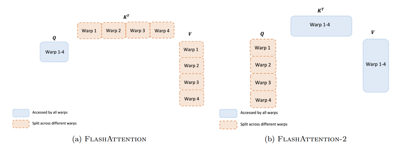
The original FlashAttention used a loop order where the outer loop iterated over $K, V$ blocks and the inner loop over $Q$ blocks. This minimized repeated loads of $K$ and $V$ from HBM, but required writing partial results to the output accumulator $O$ back to HBM after each step. This “Split-K” style (accumulating results across $K$) creates dependencies that are difficult to parallelize without atomic updates, particularly when multiple warps share the same output.
FlashAttention-2 inverts this loop hierarchy. Specifically:
- FlashAttention v1: Outer Loop ($K, V$), Inner Loop ($Q$).
- FlashAttention-2: Outer Loop ($Q$), Inner Loop ($K, V$).
Let us divide $Q$ into $T_r$ blocks and $K, V$ into $T_c$ blocks. In FlashAttention-2, a thread block loads a specific block $Q_i$ into SRAM. It then iterates through all blocks of keys and values ($K_1, V_1$ to $K_{T_c}, V_{T_c}$) (as shown in the above Figure). Since $Q_i$ is fixed for the duration of the inner loop, the corresponding output block $O_i$ is also fixed. The thread block can maintain $O_i$ entirely in registers (the fastest memory) throughout the entire computation. There is no need for atomic additions or synchronization between thread blocks regarding the output, as they write to disjoint regions of HBM. The algorithm accumulates the results of $Q_i \times K_j^\top \times V_j$ directly into registers. Only after the inner loop finishes (all $K, V$ processed) is the final result $O_i$ written to HBM. This simplifies control flow, improves memory coalescing, and completely eliminates the need to write partial results to HBM and read them back, ensuring that $O$ is written exactly once.
Optimization 3: Sequence Parallelism and Warp Partitioning
Sequence Parallelism: FlashAttention-2 solves the low occupancy issue by introducing parallelism over the sequence length dimension. Instead of assigning one thread block per attention head, v2 assigns thread blocks to chunks of the sequence. With an outer loop over $Q$ blocks, we can treat each block $Q_i$ as an independent unit of work.
For example, if the sequence length $N=8192$ and the block size $B_r = 128$, there are $T_r = 64$ blocks of $Q$.
- For a single head, we can now launch 64 thread blocks.
- For 12 heads, we launch $12 \times 64 = 768$ thread blocks.
This approach easily saturates the 108 SMs of an A100, even with a batch size of 1, ensuring high occupancy and utilization regardless of input dimensions.
Improved Warp Partitioning: A major innovation in v2 is parallelizing across the sequence dimension. Instead of one thread block handling one $(i,j)$ pair at a time, FlashAttention-2 splits the work of a single attention head into multiple thread blocks and warps.
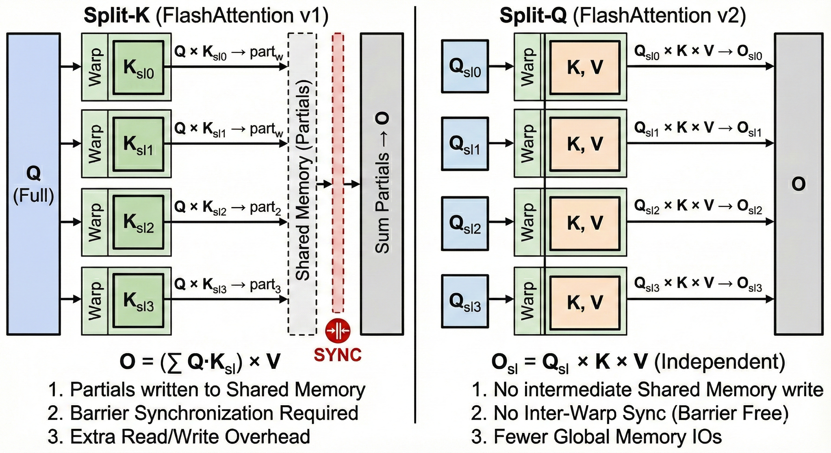
FlashAttention v1 used a “Split-K” scheme where 4 warps each computed a slice of $K^{T}$ and then synchronized to aggregate results. This required writing intermediate results to shared memory, barrier synchronization across warps, and reading/summing partial results.
In v2, the work within a thread block is partitioned differently. Since the outer loop is over $Q$, the thread block is responsible for a block of rows of $Q$. This “Split-Q” scheme allows warps to partition $Q$ instead of $K/V$. Each warp works on a disjoint slice of the output $O$, eliminating the need for inter-warp communication or synchronization.
Optimization 4: Causal Masking
In autoregressive modeling, position $i$ cannot attend to position $j$ if $j > i$. Standard attention creates a mask matrix (setting values to $-\infty$) and applies it. FlashAttention-2 optimizes this at the block level:
- Full Mask: If a block $K_j$ is entirely “future” relative to $Q_i$ (i.e., all column indices $>$ all row indices), the algorithm skips the inner loop iteration entirely. This essentially halves the compute for causal attention.
- Partial Mask: If the block lies on the diagonal (contains both valid and invalid interactions), the mask is applied on-the-fly in registers during the computation of $S_{ij}$, setting invalid entries to $-\infty$ before the softmax exponential.
Skipping blocks where all column indices exceed row indices removes about 50% of blocks for long sequences, yielding about 1.7–1.8× extra speedup.
Performance Analysis
Forward Pass
FlashAttention-2 consistently achieves ~2x the throughput of v1 and reaches high hardware utilization.
| Implementation | 2k SeqLen Speed | 8k SeqLen Speed | 16k SeqLen Speed | Note |
|---|---|---|---|---|
| Standard Attention | ~40 TFLOPs/s | OOM | OOM | Limited by HBM bandwidth. |
| FlashAttention v1 | ~110 TFLOPs/s | ~120 TFLOPs/s | ~125 TFLOPs/s | Limited by work partitioning. |
| FlashAttention-2 | ~200 TFLOPs/s | ~220 TFLOPs/s | ~225 TFLOPs/s | Near linear scaling. |
Table 1: Forward pass throughput (FP16) on A100 GPU (Head Dim 128).
Reaching 225 TFLOPs/s on a device with a theoretical max of ~312 TFLOPs/s (approx. 73% utilization) is high for a complex operation involving exponentials and reductions. Typical optimized GEMM kernels reach 80-90%, so this indicates highly effective latency hiding.
Backward Pass
FlashAttention-2 optimizes the backward pass by applying the same “Split-Q” logic. It partitions the warps to minimize synchronization when accumulating into $dK_j$ and $dV_j$, which reside in SRAM/Registers during the loop.
| Implementation | Speed (TFLOPs/s) | Theoretical Utilization |
|---|---|---|
| FlashAttention v1 | ~85 | ~27% |
| FlashAttention-2 | ~165 | ~53% |
Table 2: Backward pass throughput comparison.
While the backward pass remains slower than the forward pass (due to more FLOPs and atomic operations for $dQ$), v2 still delivers a nearly 2x improvement over v1. The bottleneck remains the atomic accumulations for $dQ$ and the higher ratio of non-matmul operations.
FlashAttention V3
FlashAttention-3 (FA3), presented at NeurIPS 2024, represents a shift in how attention kernels interact with GPU hardware. While FA1 and FA2 focused on memory hierarchy optimization (tiling) and parallelism, FA3 was designed specifically to exploit the asynchronous execution model of NVIDIA’s Hopper (H100) architecture.
Shortcomings in FA1 and FA2 on Hopper
Despite their success, FA1 and FA2 left performance potential on the table when running on modern hardware. FA2 achieves only ~35% of the theoretical maximum FLOPS on H100 GPUs, compared to 80-90% for optimized GEMM kernels
- Synchronous Execution Model: FA2 used Ampere’s
mma.syncinstruction. Hopper’s new WGMMA (Warp-Group Matrix Multiply-Accumulate) instruction achieves 50% higher throughput but requires asynchronous programming. - No Producer-Consumer Overlap: FA2’s data loading and computation were serialized. Hopper’s TMA (Tensor Memory Accelerator) enables loading the next tile while computing on the current one.
- Non-GEMM Bottleneck: H100’s Tensor Cores deliver 989 TFLOPS for FP16 matmul but only 3.9 TFLOPS for special functions (exponential). This 256× throughput gap means softmax can consume ~50% of execution time despite having far fewer FLOPs.
Improvements over FA1 & FA2
FlashAttention-3 addresses these bottlenecks through three key innovations: Warp Specialization, GEMM-Softmax Pipelining, and Low-Precision Block Quantization.
1. Warp Specialization: Producer-Consumer Model
FA3 splits the warps in a thread block into two specialized groups with distinct responsibilities, leveraging Hopper’s asynchronous nature:
- Producer Warps: exclusively issue TMA instructions to load data from global memory into a circular buffer in shared memory. Since TMA is asynchronous, a single warp can keep the memory pipeline full. For a deeper dive into TMA, see the CUTLASS tutorial
or Modal’s hardware glossary . - Consumer Warps: exclusively execute WGMMA and softmax instructions. They never issue memory loads.
This separation allows for true hardware-level parallelism. While consumer warps compute on stage $i$, producer warps load stage $(i+s) \mod s$ in parallel. Additionally, FA3 utilizes the setmaxnreg instruction for dynamic register reallocation. Producer warps need few registers, while consumer warps need many for accumulators. The hardware allows reallocating registers from producers to consumers to maximize occupancy.
2. GEMM-Softmax Pipelining (Pingpong Scheduling)
To break the sequential dependency bottleneck ($GEMM \rightarrow Softmax \rightarrow GEMM$), FA3 introduces Pingpong Scheduling between warpgroups:
- Iteration $j$: Warpgroup 1 executes the high-throughput GEMMs for blocks $j$ and $j+1$.
- Simultaneously: Warpgroup 2 executes the low-throughput Softmax for block $j-1$ on the Multi-Function Unit (MUFU), which is separate from Tensor Cores.
Intra-Warpgroup Pipelining (2-Stage Pipeline): Beyond producer-consumer overlap, FA3 pipelines execution within each consumer warpgroup. By reordering instructions, the WGMMA for the next iteration can be issued before the Softmax of the current iteration completes. This 2-stage pipeline hides the latency of the non-GEMM operations and is the precursor to the more complex 5-stage pipeline seen in FA4.
3. Low-Precision with Block Quantization
FA3 is the first to effectively utilize FP8 (8-bit floating point) for attention. However, this introduces two challenges:
Challenge 1: Layout Constraints. FP8 WGMMA requires operands in K-major format. However, for the second GEMM ($P \times V$), $V$ is typically row-major.
- Solution: FA3 performs an in-kernel transpose using
ldmatrix/stmatrixinstructions in the producer warpgroup, overlapped with the preceding GEMMs.
Challenge 2: Quantization Error. FP8 (E4M3) has only 3 mantissa bits, making it sensitive to outliers.
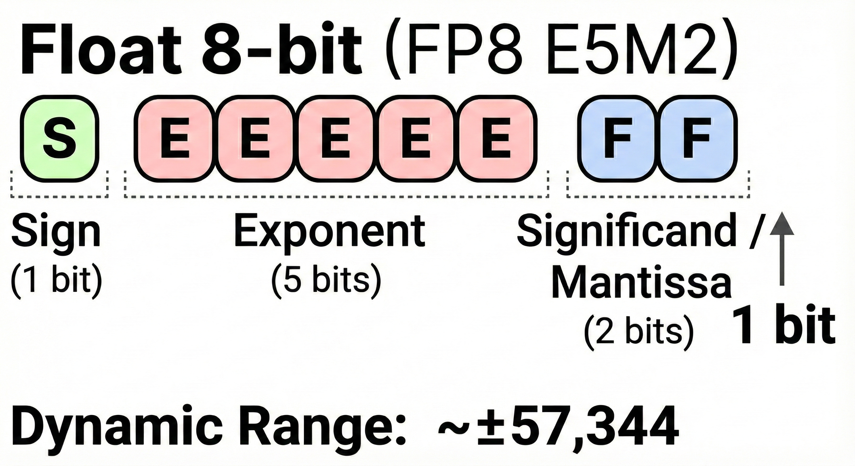
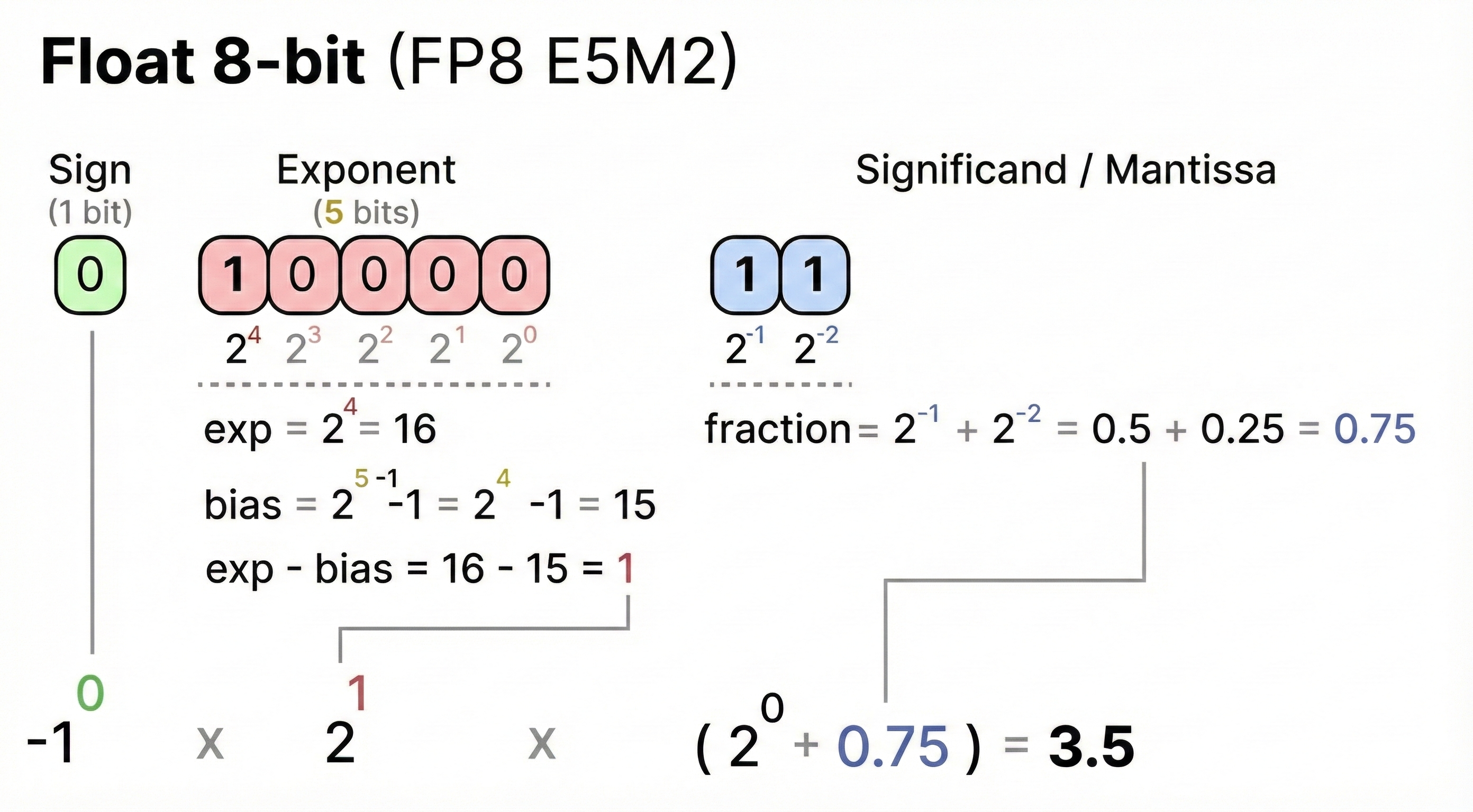
- Solution: FA3 uses Block Quantization (per-block scaling factors) and Incoherent Processing (Hadamard transform) to spread outliers.
Performance Results
On H100 GPUs, these optimizations yield significant gains:
| Configuration | FlashAttention-2 | FlashAttention-3 | Speedup |
|---|---|---|---|
| FP16 Forward | 350 TFLOPS | 740 TFLOPS | 2.1x |
| FP8 Forward | N/A | 1,200+ TFLOPS | - |
| GPU Utilization | 35% | 75-85% | 2.2x |
FlashAttention V4
FlashAttention 4 (FA4) was developed to optimize the attention mechanism for NVIDIA’s Blackwell (SM10) GPU architecture and address key architectural bottlenecks that emerged as GPUs became faster and more specialized.
Even though no official paper has been released yet, we gathered information from sources such as GPU Mode’s “How FlashAttention 4 works”
The necessity for FA4 arose because, while previous FlashAttention versions (FA1-FA3) optimized for memory movement and initial fusion, FA4 needed to shift its focus toward execution flow, sophisticated pipeline architectures, and new numerical computation techniques tailored for the Blackwell microarchitecture
1. Increased Asynchronous Pipeline (2-Stage → 5-Stage)
FlashAttention-3 relied on a simpler producer/consumer model using asynchronous memory loads (TMA) and asynchronous matrix multiplications (MMA) to achieve some latency hiding. FA4 expands this internal concurrency dramatically by mapping chunks of the pipeline onto five distinct, specialized warps: Load, MMA, Softmax, Correction, and Store.
This high level of specialization and manual concurrency management is crucial for keeping the Tensor Cores continuously busy. It represents a significant increase in complexity over the FA3 pipeline, ensuring that different parts of the GPU are utilized simultaneously without waiting for one another.
2. Software-Simulated Exponentiation (Softmax Warps)
One of the optimizations in FlashAttention 4 is not new at all; it has a direct precedent in a 25-year-old academic paper. In 1999, N. N. Schraudolph published “a fast, compact approximation of the exponential function”
Modern GPUs contain Special Function Units (SFUs), which are dedicated hardware circuits designed to accelerate transcendental math operations like the exponential function. However, FlashAttention 4 revealed that these specialized SFUs become a performance bottleneck. There are far fewer SFUs than general-purpose CUDA cores on a GPU’s streaming multiprocessor. When thousands of threads simultaneously request an exponential calculation for the softmax function, the SFUs become overloaded, leading to stalls. On Blackwell GPUs, this bottleneck can be so significant that for a common configuration, the softmax computation takes approximately twice as long (1024 cycles) as each of the two main matrix multiplications (512 cycles each).
FA4 addresses this by moving the exponential calculation onto the general-purpose CUDA Cores using dedicated Softmax warps. The calculation approximates $2^x = 2^i \cdot 2^f$ by:
- Using a cubic polynomial approximation $P(f)$ for the fractional part $2^f$, often performed using three fused multiply-adds (FMA).
- Scaling by the integer part $2^i$ through adding the integer $i$ directly to the exponent field of the floating-point number, rather than requiring a full multiplication.
This software-based approach allows the kernel to compute two exponential values simultaneously, doubling the parallelism of this step and bypassing the SFU bottleneck entirely.
3. Selective Rescaling (Correction Warps)
To maintain numerical stability during the attention calculation, kernels must frequently rescale intermediate values. Traditionally, this happens every time a new maximum score is found. Each rescaling operation requires a synchronization point, which introduces coordination overhead. In FA4’s highly asynchronous pipeline, where different warps handle loading, computation, and correction simultaneously, these synchronization events are particularly costly as they can force the entire pipeline to halt and wait.
FlashAttention 4, through its specialized Correction warps, adopts a selective approach: selective rescaling. Instead of rescaling every time the maximum value changes, the kernel only performs the operation when the change is “significant enough to affect numerical correctness.” The impact of this change is significant, resulting in a 10x reduction in rescaling operations. Fewer rescaling operations mean fewer synchronization points and pipeline stalls, significantly reducing overhead and contributing to the kernel’s overall speed.
Mathematically, let’s define the maximum attention score utilized as the scaling factor, $m_{\text{old}}$, and the pre-defined tolerance threshold, $\epsilon$:
- $m_{\text{old}} = \text{Current Running Maximum}$
- $\epsilon = \text{Tolerance Threshold (e.g., related to machine epsilon)}$
The kernel checks if the difference between the new maximum ($m_{\text{new}}$) and the old maximum ($m_{\text{old}}$) is numerically large enough to potentially compromise precision. This is the core condition for selective rescaling:
\[\text{Difference} = \lvert m_{\text{new}} - m_{\text{old}} \rvert\]Check Condition: $\lvert m_{\text{new}} - m_{\text{old}} \rvert > \epsilon$?
Case A: No Rescaling Triggered If $\lvert m_{\text{new}} - m_{\text{old}} \rvert \le \epsilon$:
- Action: No rescaling is performed.
- Result: The previous running maximum $m_{\text{old}}$ is kept, and the kernel avoids the synchronization overhead.
Case B: Rescaling Triggered If $|m_{\text{new}} - m_{\text{old}}| > \epsilon$, rescaling is required to prevent numerical overflow and maintain precision.
- Update Maximum: The new maximum $m_{\text{new}}$ becomes the current scaling factor. \(m_{\text{old}} \leftarrow m_{\text{new}}\)
- Trigger Correction: The Softmax warps signal the Correction warps.
- Apply Correction: The Correction warps update the previously accumulated output values to maintain numerical correctness relative to the new, larger scale.
4. Blackwell Hardware Exploitation and Tensor Memory
FlashAttention 4 is purpose-built to leverage the specific architectural features of NVIDIA’s Blackwell GPUs, most notably Tensor Memory. In previous architectures, managing intermediate results often required shuffling data between registers and shared memory, creating bottlenecks. Blackwell introduces Tensor Memory as a programmer-managed L1 cache designed specifically to hold and accumulate intermediates, such as unnormalized attention scores ($S$) and output values ($O$), directly during Tensor Core operations.
The kernel utilizes the Tensor Memory Accelerator (TMA) to handle asynchronous memory loads, significantly reducing register pressure by firing off copy operations asynchronously. Furthermore, FA4 simplifies matrix operations by relying on single Cooperative Thread Array (CTA) matrix multiplications (cta_group::1). This means it no longer requires warp groups for optimal performance—a departure from the complexity required in previous generations to saturate the GPU.
5. Complete Warp Specialization Roles
While the 5-stage pipeline was introduced earlier, the true power of FA4 lies in the strict specialization of its warps. Each warp type has a singular focus, preventing resource contention and context switching overhead:
- Load Warps: These are dedicated solely to maximizing memory bandwidth. They pre-fetch Query, Key, and Value data blocks from global memory into shared memory, ensuring the compute units never starve for data.
- MMA Warps: These warps focus purely on computation. They drive the Tensor Cores to compute the partial attention score matrix ($QK^T$) and accumulate value tiles ($PV$) into the output tiles, without being burdened by memory management or control logic.
- Store/Epilogue Warps: Dedicated to the final stage of the pipeline, these warps manage the efficient transfer of accumulated output blocks from on-chip memory back to global memory, handling the necessary data layout transformations.
6. Performance Context and Current Limitations
FlashAttention 4 marks a milestone in GPU computing as the first attention kernel to break the petaflop threshold, achieving over $10^{15}$ floating-point operations per second. It reaches an efficiency of approximately 30% MFU (Model Flops Utilization), performing 5–10% to 22% faster than NVIDIA’s standard cuDNN implementation.
However, as an early release targeting a new architecture, it currently has specific limitations:
- Forward Pass Only: The current implementation supports only forward propagation, with backward pass support planned for future releases.
- BF-16 Precision: The kernel operates exclusively in BF-16 precision.
- Future Optimizations: It does not yet utilize FP4 operations or 2-CTA matrix multiplications, which are key Blackwell features that promise even greater performance gains in the future.
Principles for Future Attention Algorithms
The evolution from FlashAttention v1 through v4 reveals several core principles that extend beyond simply optimizing existing attention mechanisms. These principles form a foundation for thinking about future attention algorithms as the hardware landscape continues to evolve.
First, memory hierarchy awareness must become a first-class concern in algorithm design. The FlashAttention series demonstrates that asymptotic complexity alone is insufficient—the IO complexity term O(N²d²M⁻¹) matters as much as the FLOP count. Future attention mechanisms should be designed with explicit consideration of data movement costs across the memory hierarchy. This means algorithms cannot treat memory as a flat abstraction but must account for the multi-level nature of modern GPU memory systems.
Second, kernel fusion and recomputation trade-offs offer underexplored design space. FlashAttention’s backward pass trades additional compute for reduced memory traffic, exploiting the fact that modern accelerators are increasingly memory-bound rather than compute-bound. This suggests a broader principle: as the compute-to-bandwidth ratio continues to grow in future hardware, selectively recomputing intermediate values rather than storing them becomes increasingly favorable. The question becomes which intermediate tensors to materialize and which to recompute, a decision that depends on both the operation’s arithmetic intensity and its position in the dependency graph.
Third, hardware-algorithm co-design requires specialization at the warp level. FlashAttention v3 and v4’s progression toward fine-grained warp specialization—separating producer, consumer, and correction roles—suggests that future kernels must exploit asynchronous execution models more aggressively. The trend toward heterogeneous functional units (Tensor Cores, SFUs, CUDA cores) means algorithms should explicitly partition work to match the throughput characteristics of each unit type, rather than treating the GPU as a homogeneous compute resource.
Finally, numerical precision is a tunable parameter, not a fixed constraint. FlashAttention-3’s block quantization and FA4’s software-based exponential approximation demonstrate that carefully managed low-precision computation can maintain accuracy while improving throughput. Future algorithms might adaptively select precision per-operation based on numerical sensitivity analysis, potentially using FP8 or FP4 for matmuls while maintaining higher precision only where gradients demand it.
These principles point toward a future where attention mechanisms are not merely approximate variants of the standard formulation, but fundamentally redesigned algorithms that achieve exact results through hardware-conscious implementation strategies.
Appendix A: Standard Attention Complexity
The standard self-attention mechanism in Transformers is formally defined as:
\[\text{Attention}(Q, K, V) = \text{softmax}\left(\frac{QK^T}{\sqrt{d_k}}\right)V\]where inputs $Q, K \in \mathbb{R}^{n \times d_k}$ and $V \in \mathbb{R}^{n \times d_v}$ represent the query, key, and value matrices respectively. The computation proceeds in three sequential stages, each contributing to the overall computational cost.
First, we compute the attention score matrix $S = \frac{QK^T}{\sqrt{d_k}}$. This operation involves a matrix multiplication between $Q$ and $K^T$, resulting in an $n \times n$ matrix. Since each of the $n^2$ entries requires a dot product of size $d_k$, the computational cost is proportional to the number of elements multiplied by the dimension size.
\[\text{Time Complexity (Scores)} = O(n^2 d_k)\]Crucially, this step requires storing the intermediate matrix $S$, which scales quadratically with the sequence length $n$. This $O(n^2)$ memory requirement is the primary bottleneck for long sequences.
Second, we apply the softmax function row-wise to normalize the scores. For each of the $n$ rows, we compute exponentials, sum them, and divide to normalize. As this is performed for every element in the $n \times n$ matrix, the cost is quadratic.
\[\text{Time Complexity (Softmax)} = O(n^2)\]Finally, we compute the weighted sum of values by multiplying the normalized probability matrix $P = \text{softmax}(S)$ with the value matrix $V$. This results in an output matrix of size $n \times d_v$. Similar to the first step, each of the $n \times d_v$ output elements requires a dot product of length $n$.
\[\text{Time Complexity (Aggregation)} = O(n^2 d_v)\]Summing these components gives the total time complexity:
\[\text{Total Time} = O(n^2 d_k) + O(n^2) + O(n^2 d_v) = O(n^2(d_k + d_v))\]In typical Transformer architectures, the head dimensions $d_k$ and $d_v$ are proportional to the model dimension $d_{\text{model}}$. Thus, the complexity is often simplified to $O(n^2 d_{\text{model}})$.
Scalability Implications
The quadratic dependency on sequence length $n$ creates significant resource challenges as context length increases. The table below illustrates how computational cost and memory usage grow with sequence length, assuming a hidden dimension of $d=768$.
| Sequence Length | Relative Compute Cost | Memory (GB) |
|---|---|---|
| 512 | 1× | 0.001 |
| 2,048 | 16× | 0.016 |
| 8,192 | 256× | 0.25 |
| 65,536 | 16,384× | 16 |
| 1M | 4,000,000× | 4,000 |
Theoretical Lower Bounds
One might ask if it is possible to compute attention more efficiently than $O(n^2)$. Research grounded in the Strong Exponential Time Hypothesis (SETH) suggests that this quadratic cost is fundamental. Specifically, it has been proven that for any $\epsilon > 0$, computing the softmax dot-product attention requires $\Omega(n^{2-\epsilon})$ time.
This lower bound holds for exact computation as well as for multiplicative and additive approximations. The proof relies on a reduction from the Orthogonal Vectors Problem (OVP). Intuitively, to accurately determine the attention distribution, the algorithm must evaluate pairwise interactions between query and key vectors. In high-dimensional spaces, distinguishing between orthogonal and nearly-orthogonal vectors requires checking all pairs, which establishes the $\Omega(n^2)$ barrier.
Appendix B: Memory Bound Proof
We prove that standard attention is memory-bound by analyzing the Arithmetic Intensity ($AI$) of its components. An operation is memory-bound if its $AI$ is lower than the hardware’s critical threshold ($I_{crit}$). For an NVIDIA A100, $I_{crit} \approx 12.5$ FLOPs/Byte.
Standard attention consists of three kernels:
- MatMul 1 ($S = QK^T$): Compute-bound ($AI \approx 64$ for $d=64$).
- Softmax ($P = \text{softmax}(S)$): Memory-bound.
- MatMul 2 ($O = PV$): Compute-bound ($AI \approx 64$).
Analysis of the Softmax Kernel:
- Compute: Softmax performs element-wise operations (exp, sum, div) on the $N \times N$ matrix. This requires approximately 5 FLOPs per element. \(\text{FLOPs} \approx 5N^2\)
- Memory: The kernel must read the full matrix $S$ from HBM and write the full matrix $P$ back to HBM. For FP16 precision ($P=2$ bytes), the data movement is: \(\text{Bytes} = 2 \times (N^2 \text{ read} + N^2 \text{ write}) = 4N^2\)
- Arithmetic Intensity: \(AI_{\text{softmax}} = \frac{5N^2}{4N^2} = 1.25 \text{ FLOPs/Byte}\)
Conclusion: Since $1.25 \ll 12.5$, the Softmax kernel is severely memory-bound. It forces the GPU compute cores to stall while waiting for $O(N^2)$ data to move to and from HBM. Therefore, despite the high compute complexity of the matrix multiplications, the intermediate materialization of the attention matrix creates a bandwidth bottleneck that limits overall performance.