The Illustrated MicroGPT: A Dependency-Free GPT from Scratch
In this post, we’re going to dissect a piece of educational code: MicroGPT. Written by Andrej Karpathy, this script trains and runs a GPT language model using pure Python. No PyTorch, no TensorFlow, no NumPy. Just raw Python standard library.
The original code can be found here.
“I thought about it more and realized that the autograd engine can be even more dramatically simplified. 243 lines of code is now down to 200, ~18% reduction. Surely this is it now!” — Andrej Karpathy
Let’s walk through it, block by block, illustrating how everything works.
1. The Setup
First, we import the necessary standard libraries. math for mathematical operations, and random for generating numbers.
import os       # os.path.exists
import math     # math.log, math.exp
import random   # random.seed, random.choices, random.gauss, random.shuffle
random.seed(42) # Let there be order among chaos
Setting random.seed(42) ensures that every time we run this code, we get the exact same sequence of random numbers. This is crucial for reproducibility and debugging.
2. The Data Pipeline
We need text to train on. Here, we check for input.txt. If it’s missing, we download a dataset of names.
# Let there be an input dataset `docs`: list[str] of documents (e.g. a dataset of names)
if not os.path.exists('input.txt'):
    import urllib.request
    names_url = 'https://raw.githubusercontent.com/karpathy/makemore/refs/heads/master/names.txt'
    urllib.request.urlretrieve(names_url, 'input.txt')
docs = [l.strip() for l in open('input.txt').read().strip().split('\n') if l.strip()] # list[str] of documents
random.shuffle(docs)
print(f"num docs: {len(docs)}")
# num docs: 32033
Tokenization: Strings to Integers
Neural networks don’t understand “A”; they understand 1. This section builds a vocabulary (list of unique characters) and mappings between characters and integers.
# Let there be a Tokenizer to translate strings to discrete symbols and back
uchars = sorted(set(''.join(docs))) # unique characters in the dataset become token ids 0..n-1
BOS = len(uchars) # token id for the special Beginning of Sequence (BOS) token
vocab_size = len(uchars) + 1 # total number of unique tokens, +1 is for BOS
print(f"vocab size: {vocab_size}")
# vocab size: 27
What’s happening here?

We also add a special token <BOS> (Beginning of Sequence) to mark the start and end of names.
3. The Engine: Autograd via Value
To train a neural network, we need gradients—we need to know how much to nudge each weight to reduce the error. Since we don’t have PyTorch, Karpathy implements a tiny engine to do this manually.
The Value class wraps a number (data) and tracks its gradient (grad). Instead of storing full backward closures, this new version simply stores local_grads—the derivative of the node with respect to its children.
# Let there be an Autograd to apply the chain rule recursively across a computation graph
class Value:
    """Stores a single scalar value and its gradient, as a node in a computation graph."""

    def __init__(self, data, children=(), local_grads=()):
        self.data = data                # scalar value of this node calculated during forward pass
        self.grad = 0                   # derivative of the loss w.r.t. this node, calculated in backward pass
        self._children = children       # children of this node in the computation graph
        self._local_grads = local_grads # local derivative of this node w.r.t. its children

    def __add__(self, other):
        other = other if isinstance(other, Value) else Value(other)
        return Value(self.data + other.data, (self, other), (1, 1))

    def __mul__(self, other):
        other = other if isinstance(other, Value) else Value(other)
        return Value(self.data * other.data, (self, other), (other.data, self.data))

    def __pow__(self, other): return Value(self.data**other, (self,), (other * self.data**(other-1),))
    def log(self): return Value(math.log(self.data), (self,), (1/self.data,))
    def exp(self): return Value(math.exp(self.data), (self,), (math.exp(self.data),))
    def relu(self): return Value(max(0, self.data), (self,), (float(self.data > 0),))
    def __neg__(self): return self * -1
    def __radd__(self, other): return self + other
    def __sub__(self, other): return self + (-other)
    def __rsub__(self, other): return other + (-self)
    def __rmul__(self, other): return self * other
    def __truediv__(self, other): return self * other**-1
    def __rtruediv__(self, other): return other * self**-1

    def backward(self):
        topo = []
        visited = set()
        def build_topo(v):
            if v not in visited:
                visited.add(v)
                for child in v._children:
                    build_topo(child)
                topo.append(v)
        build_topo(self)
        self.grad = 1
        for v in reversed(topo):
            for child, local_grad in zip(v._children, v._local_grads):
                child.grad += local_grad * v.grad
Visualizing the Computation Graph Node:
When you do c = a + b, a graph is created:

When we call c.backward(), the gradients flow backwards:
-
c.gradstarts at 1.0. - The
backwardmethod iterates through the graph in reverse topological order. - It accumulates gradients using
local_grads(child.grad += local_grad * v.grad).
4. Initializing the Model
Here we define the transformer’s hyperparameters and initialize the weights (parameters) with random values.
# Initialize the parameters, to store the knowledge of the model.
n_embd = 16     # embedding dimension
n_head = 4      # number of attention heads
n_layer = 1     # number of layers
block_size = 8  # maximum sequence length
head_dim = n_embd // n_head # dimension of each head
matrix = lambda nout, nin, std=0.02: [[Value(random.gauss(0, std)) for _ in range(nin)] for _ in range(nout)]
state_dict = {'wte': matrix(vocab_size, n_embd), 'wpe': matrix(block_size, n_embd), 'lm_head': matrix(vocab_size, n_embd)}
for i in range(n_layer):
    state_dict[f'layer{i}.attn_wq'] = matrix(n_embd, n_embd)
    state_dict[f'layer{i}.attn_wk'] = matrix(n_embd, n_embd)
    state_dict[f'layer{i}.attn_wv'] = matrix(n_embd, n_embd)
    state_dict[f'layer{i}.attn_wo'] = matrix(n_embd, n_embd, std=0)
    state_dict[f'layer{i}.mlp_fc1'] = matrix(4 * n_embd, n_embd)
    state_dict[f'layer{i}.mlp_fc2'] = matrix(n_embd, 4 * n_embd, std=0)
params = [p for mat in state_dict.values() for row in mat for p in row] # flatten params into a single list[Value]
print(f"num params: {len(params)}")
# num params: 4064
Key Parameters:
-
wte: Token Embeddings (Lookup table for characters) -
wpe: Position Embeddings (Lookup table for positions 0, 1, 2…) -
attn_w*: Attention weights (Query, Key, Value, Output) -
mlp_fc*: Feed-Forward Network weights
5. The Model Architecture
This is the heart of GPT. It consists of layers (just 1 here), each having Self-Attention and a Multi-Layer Perceptron (MLP).
# Define the model architecture: a stateless function mapping token sequence and parameters to logits over what comes next.
# Follow GPT-2, blessed among the GPTs, with minor differences: layernorm -> rmsnorm, no biases, GeLU -> ReLU^2
def linear(x, w):
    return [sum(wi * xi for wi, xi in zip(wo, x)) for wo in w]

def softmax(logits):
    max_val = max(val.data for val in logits)
    exps = [(val - max_val).exp() for val in logits]
    total = sum(exps)
    return [e / total for e in exps]

def rmsnorm(x):
    ms = sum(xi * xi for xi in x) / len(x)
    scale = (ms + 1e-5) ** -0.5
    return [xi * scale for xi in x]

def gpt(token_id, pos_id, keys, values):
    tok_emb = state_dict['wte'][token_id] # token embedding
    pos_emb = state_dict['wpe'][pos_id] # position embedding
    x = [t + p for t, p in zip(tok_emb, pos_emb)] # joint token and position embedding
    x = rmsnorm(x)

    for li in range(n_layer):
        # 1) Multi-head attention block
        x_residual = x
        x = rmsnorm(x)
        q = linear(x, state_dict[f'layer{li}.attn_wq'])
        k = linear(x, state_dict[f'layer{li}.attn_wk'])
        v = linear(x, state_dict[f'layer{li}.attn_wv'])
        keys[li].append(k)
        values[li].append(v)
        x_attn = []
        for h in range(n_head):
            hs = h * head_dim
            q_h = q[hs:hs+head_dim]
            k_h = [ki[hs:hs+head_dim] for ki in keys[li]]
            v_h = [vi[hs:hs+head_dim] for vi in values[li]]
            attn_logits = [sum(q_h[j] * k_h[t][j] for j in range(head_dim)) / head_dim**0.5 for t in range(len(k_h))]
            attn_weights = softmax(attn_logits)
            head_out = [sum(attn_weights[t] * v_h[t][j] for t in range(len(v_h))) for j in range(head_dim)]
            x_attn.extend(head_out)
        x = linear(x_attn, state_dict[f'layer{li}.attn_wo'])
        x = [a + b for a, b in zip(x, x_residual)]
        # 2) MLP block
        x_residual = x
        x = rmsnorm(x)
        x = linear(x, state_dict[f'layer{li}.mlp_fc1'])
        x = [xi.relu() ** 2 for xi in x]
        x = linear(x, state_dict[f'layer{li}.mlp_fc2'])
        x = [a + b for a, b in zip(x, x_residual)]

    logits = linear(x, state_dict['lm_head'])
    return logits
The Architecture Flow:

Attention Mechanism:

The attention block (sections calculating q, k, v) allows the model to look back at previous tokens. It asks: “Given what I am (Query), what information from the past (Keys) is relevant to me?” and then aggregates that information (Values).
Understanding Softmax:

Softmax takes raw scores (logits) and turns them into probabilities that sum to 1. It amplifies the largest value, making it the “winner”.
6. Training the Model
We use Adam optimization. In a loop, we grab a document, run the model forward to get a loss (error), backpropagate to find gradients, and update the weights. We also use a cosine learning rate decay schedule, which gradually lowers the learning rate to help the model converge more smoothly.
# Let there be Adam, the blessed optimizer and its buffers
learning_rate, beta1, beta2, eps_adam = 1e-2, 0.9, 0.95, 1e-8
m = [0.0] * len(params) # first moment buffer
v = [0.0] * len(params) # second moment buffer

# Repeat in sequence
num_steps = 500 # number of training steps
for step in range(num_steps):

    # Take single document, tokenize it, surround it with BOS special token on both sides
    doc = docs[step % len(docs)]
    tokens = [BOS] + [uchars.index(ch) for ch in doc] + [BOS]
    n = min(block_size, len(tokens) - 1)

    # Forward the token sequence through the model, building up the computation graph all the way to the loss.
    keys, values = [[] for _ in range(n_layer)], [[] for _ in range(n_layer)]
    losses = []
    for pos_id in range(n):
        token_id, target_id = tokens[pos_id], tokens[pos_id + 1]
        logits = gpt(token_id, pos_id, keys, values)
        probs = softmax(logits)
        loss_t = -probs[target_id].log()
        losses.append(loss_t)
    loss = (1 / n) * sum(losses) # final average loss over the document sequence. May yours be low.

    # Backward the loss, calculating the gradients with respect to all model parameters.
    loss.backward()

    # Adam optimizer update: update the model parameters based on the corresponding gradients.
    lr_t = learning_rate * 0.5 * (1 + math.cos(math.pi * step / num_steps)) # cosine learning rate decay
    for i, p in enumerate(params):
        m[i] = beta1 * m[i] + (1 - beta1) * p.grad
        v[i] = beta2 * v[i] + (1 - beta2) * p.grad ** 2
        m_hat = m[i] / (1 - beta1 ** (step + 1))
        v_hat = v[i] / (1 - beta2 ** (step + 1))
        p.data -= lr_t * m_hat / (v_hat ** 0.5 + eps_adam)
        p.grad = 0

    print(f"step {step+1:4d} / {num_steps:4d} | loss {loss.data:.4f}")
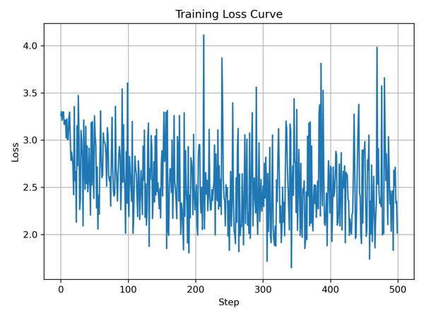
Training Results:
After running the training loop for 500 steps, we see the loss decrease significantly:
- Initial loss: 3.262670
- Final loss: 2.015951
The Training Cycle:

7. Inference: Let it Speak
Finally, we let the model generate new names! We start with the <BOS> token and ask the model to predict the next character, feeding it back in until we hit <BOS> again (end of name).
# Inference: may the model babble back to us
temperature = 0.5 # in (0, 1], control the "creativity" of generated text, low to high
print("\n--- inference ---")
for sample_idx in range(20):
    keys, values = [[] for _ in range(n_layer)], [[] for _ in range(n_layer)]
    token_id = BOS
    sample = []
    for pos_id in range(block_size):
        logits = gpt(token_id, pos_id, keys, values)
        probs = softmax([l / temperature for l in logits])
        token_id = random.choices(range(vocab_size), weights=[p.data for p in probs])[0]
        if token_id == BOS:
            break
        sample.append(uchars[token_id])
    print(f"sample {sample_idx+1:2d}: {''.join(sample)}")
Output:
--- inference ---
sample 1: lellen
sample 2: keles
sample 3: aylera
sample 4: kellone
sample 5: aman
sample 6: lela
sample 7: ameri
sample 8: kan
sample 9: nareena
sample 10: aliela
sample 11: seyn
sample 12: daman
sample 13: caaren
sample 14: ozyren
sample 15: kahiea
sample 16: anytte
sample 17: shilol
sample 18: deler
sample 19: azele
sample 20: maton
And there you have it. A complete, trainable, inferencable GPT model in pure Python. It demystifies the black box, showing that at their core, these massive AI models are just a series of matrix multiplications and gradients.
Enjoy Reading This Article?
Here are some more articles you might like to read next: