Transformers:Self Attention Mechanism

The transformer is one of the most popular state-of-the-art deep learning architectures that is mostly used for natural language processing (NLP) tasks. Ever since the advent of the transformer, it has replaced the recurrent neural network (RNN) and long short-term memory (LSTM) for various tasks. Several new NLP models, such as BERT, GPT, and T5, are based on the transformer architecture.

RNN and LSTM networks are widely used in sequential tasks such as next word prediction, machine translation, text generation, and more. However, one of the major challenges with the recurrent model is capturing the long-term dependency.

To overcome this limitation of RNNs, a new architecture called Transformer was introduced in the paper “Attention Is All You Need.” The transformer is currently the state-of-the-art model

The transformer model is based entirely on the attention mechanism and completely gets rid of recurrence. The transformer uses a special type of attention mechanism called self-attention.

How does the transformer work ?

Let’s understand how the transformer works with a language translation task. The transformer consists of an encoder-decoder architecture. We feed the input sentence (source sentence) to the encoder. The encoder learns the representation of the input sentence and sends the representation to the decoder. The decoder receives the representation learned by the encoder as an input and generates the output sentence (target sentence).
Suppose we need to convert a sentence from English to French. We feed the English sentence as input to the encoder. The encoder learns the representation of the given English sentence and feeds the representation to the decoder. The decoder takes the encoder’s representation as input and generates the French sentence as output

Okay, but what’s exactly going on here? How does the encoder and decoder in the transformer convert the English sentence (source sentence) to the French sentence (target sentence)? What’s going on inside the encoder and decoder?

Understanding the Encoder of the Transformer

The transformer consists of a stack of 𝑁 number of encoders. The output of one encoder is sent as input to the encoder above it. As shown in the following figure, we have a stack of 𝑁 number of encoders. Each encoder sends its output to the encoder above it. The final encoder returns the representation of the given source sentence as output. We feed the source sentence as input to the encoder and get the representation of the source sentence as output:

Note that in the transformer paper “Attention Is All You Need_,”_ the authors have used 𝑁=6, meaning that they stacked up six encoders, one above the other. However, we can try out different values of 𝑁.

Lets Keep N=2 for simplicity

Encoder’s Components

Okay, the question is, how exactly does the encoder work? How is it generating the representation for the given source sentence (input sentence)? To understand this, let’s tap into the encoder and see its components. The following figure shows the components of the encoder

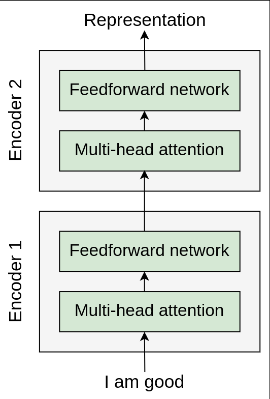
From the preceding figure, we can understand that all the encoder blocks are identical. We can also observe that each encoder block consists of two sublayers:

• Multi-head attention

• Feedforward network

To understand how multi-head attention works, we first need to understand the self-attention mechanism.

Self Attention Mechanism

Let’s understand the self-attention mechanism with an example. Consider the following sentence:

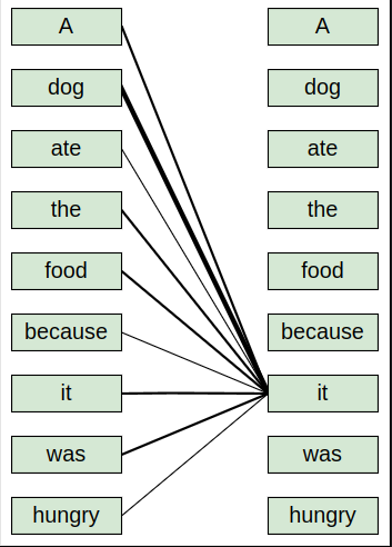
A dog ate the food because it was hungry

In the preceding sentence, the pronoun ‘it’ could mean either ‘dog’ or ‘food’. By reading the sentence, we can easily understand that the pronoun ‘it’ implies the ‘dog’ and not ‘food’. But how does our model understand that in the given sentence, the pronoun ‘it’ implies the ‘dog’ and not ‘food’? Here is where the self-attention mechanism helps us.

Representation of the words

In the given sentence, ‘A dog ate the food because it was hungry’, first our model computes the representation of the word ‘A’, next it computes the representation of the word ‘dog’, then it computes the representation of the word ‘ate’, and so on. While computing the representation of each word, it relates each word to all other words in the sentence to understand more about the word.

Computing the representation of the words

For instance, while computing the representation of the word ‘it’, our model relates the word ‘it’ to all the words in the sentence to understand more about the word ‘it’.

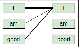
As shown in the following figure, in order to compute the representation of the word ‘it’, our model relates the word ‘it’ to all the words in the sentence. By relating the word ‘it’ to all the words in the sentence, our model can understand that the word ‘it’ is related to the word ‘dog’ and not ‘food’. As we can observe, the line connecting the word ‘it’ to ‘dog’ is thicker compared to the other lines, which indicates that the word ‘it’ is related to the word ‘dog’ and not ‘food’ in the given sentence:

Okay, but how exactly does this work? Now that we have a basic idea of what the self-attention mechanism is, let’s understand more about it in detail.

What is embedding?

Suppose our input sentence (source sentence) is ‘I am good’. First, we get the embeddings for each word in our sentence. Note that the embeddings are just the vector representation of the word and the values of the embeddings will be learned during training.

Let $x_1$ ​ be the embedding of the word ‘I’, $x_2$ ​ be the embedding of the word ‘am’, and $x_3$ ​ be the embedding of the word ‘good’. Consider the following:

• The embedding of the word ‘I’ is $x_1$ ​=[1.76,2.22,…,6.66]
• The embedding of the word ‘am’ is $x_2$ ​=[7.77,0.631,…,5.35]
• The embedding of the word ‘good’ is $x_3$ ​=[11.44,10.10,…,3.33]

Then, we can represent our input sentence ‘I am good’ using the input matrix 𝑋X (embedding matrix or input embedding), as shown here:

Note: The values used in the preceding matrix are arbitrary and used here just to give us a better understanding.

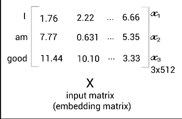
From the preceding input matrix 𝑋, we can understand that the first row of the matrix implies the embedding of the word ‘I’, the second row implies the embedding of the word ‘am’, and the third row implies the embedding of the word ‘good’.

Dimensions of the embedding matrix

The dimension of the input matrix $X$ will be $[sentencelength\ast embeddingdimension]$ The number of words in our sentence (sentence length) is 3. Let the embedding dimension be 512; then, our input matrix (input embedding) dimension will be:

$$[3\ast 512]$$

Now from the input matrix $X$, we create three new matrices; a query matrix $Q$, key matrix $K$, and a value matrix $V$. These matrices are used in the self attention mechanism

How can we create the query, key, and value matrices?

To create these, we introduce three new weight matrices called $W^Q$ , $W^K$, $W^V$ We create the query $Q$, key $K$ and value $V$ by multiplying the matrix $X$ by  $W^Q$ , $W^K$, $W^V$ respectively

Note: The weight matrices $W^Q$ , $W^K$, $W^V$  are randomly initialized, and their optimal values will be learned during training. As we learn the optimal weights, we will obtain more accurate query, key, and value matrices

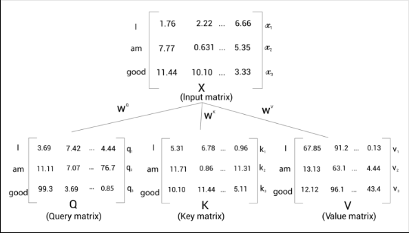
From the preceding figure, we can understand the following:

• The first row in the query, key, and value matrices— $q_1$​ ,$k_1$​, and $v_1$​—implies the query, key, and value vectors of the word ‘I’.
• The second row in the query, key, and value matrices $q_2$​​ , $k_2$​, and $v_2$​—implies the query, key, and value vectors of the word ‘am’.
• The third row in the query, key, and value matrices— $q_3$​ , $k_3$​, and $v_3$​ —implies the query, key, and value vectors of the word ‘good’.

Dimensions of the query, key and value matrices

Note that the dimensionality of the query, key, and value vectors is 64. Thus, the dimension of our query, key, and value matrices is:

$$[sentencelength\ast 64]$$

Since we have three words in the sentence, the dimensions of the query, key and value matrices are:

$$[3\ast 64]$$

But still, the ultimate question is, why are we computing this? What is the use of query, key, and value matrices? How is this going to help us?

How the self-attention mechanism works

We learned how to compute query, 𝑄 key, 𝐾, and value, 𝑉, matrices and we also learned that they are obtained from the input matrix, 𝑋. Now, let’s see how the query, key, and value matrices are used in the self-attention mechanism.

We learned that in order to compute a representation of a word, the self-attention mechanism relates the word to all the words in the given sentence. Consider the sentence ‘I am good’. To compute the representation of the word ‘I’, we relate the word ‘I’ to all the words in the sentence, as shown in the following figure:

But why do we need to do this? Understanding how a word is related to all the words in the sentence helps us to learn better representation. Now, let’s learn how the self-attention mechanism relates a word to all the words in the sentence using the query, key, and value matrices. The self-attention mechanism includes four steps. Let’s take a look at them one by one.

Step 1 : Calculating the similarity score

The first step in the self-attention mechanism is to compute the dot product between the query matrix $Q$ and the key matrix $K^T$

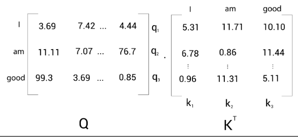
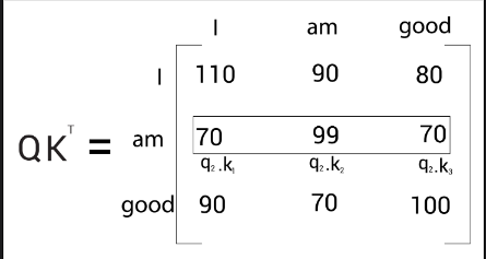
The following shows the result of the dot product between the query matrix, 𝑄, and the key matrix, $K^T$:

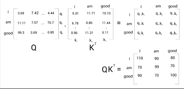But what is the use of computing the dot product between the query and key matrices? What exactly does $Q\ast K^T$ signify? Let’s understand this by looking at the result in detail.

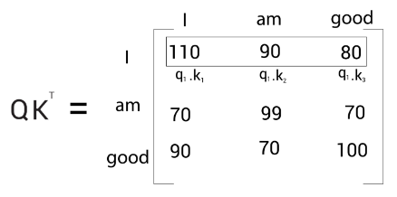
The similarity score for ‘I’

Let’s look into the first row of the $Q\ast K^T$  matrix as shown in the following figure. We can observe that we are computing the dot product between the query vector $q_1$, and all the key vectors— $k_1(I),k_2(am),k_3(good)$. Computing the dot product between two vectors tells us how similar they are.

Therefore, computing the dot product between the query vector  $q_1$ and the key vectors $k_1,k_2,k_3$ tells us how similar the query vector $q_1$  is to all the key vectors— $k_1(I),k_2(am),k_3(good)$, By looking at the first row of the $Q{K}^T$  matrix, we can understand that the word ‘I’ is more related to itself than the words ‘am’ and ‘good’ since the dot product value is higher for $q_1\ast k_1$ compared to $q_1\ast k_2$ and $q_1\ast k_3$:

Note: The values used in the input matrices are arbitrary and used here just to give us a better understanding.

The similarity score for ‘am’

Now, let’s look into the second row of the $Q\ast K^T$ matrix . As shown in the following figure, we can observe that we are computing the dot product between the query vector, $q_2(am)$ and all the key vectors— $k_1(I),k_2(am),k_3(good)$, and $k_3(good)$. This tells us how similar the query vector $q_2(am)$  is to the key vectors— $k_1(I),k_2(am),k_3(good)$ , and $k_3(good)$.

By looking at the second row of the $Q\ast K^T$ matrix, we can understand that the word ‘am’ is more related to itself than the words ‘I’ and ‘good’ since the dot product value is higher for $q_2\ast k_2$ compared to $q_2\ast k_1$ and $q_2\ast k_3$​:

The similarity score for ‘good’

Similarly, let’s look into the third row of the $Q\ast K^T$  matrix. As shown in the following figure, we can observe that we are computing the dot product between the query vector 𝑞3(good)q3​(good) and all the key vectors— $k_1(I),k_2(am),k_3(good)$. This tells us how similar the query vector 𝑞3(good)q3​(good) is to all the key vectors— $k_1(I),k_2(am),k_3(good)$. By looking at the third row of the $Q\ast K^T$ matrix, we can understand that the word ‘good’ is more related to itself than the words ‘I’ and ‘am’ in the sentence since the dot product value is higher for $q_3\ast k_3$  compared to $q_3\ast k_1$  and $q_3\ast k_2$:

Thus, we can say that computing the dot product between the query matrix 𝑄, and the key matrix $K^T$, essentially gives us the similarity score, which helps us to understand how similar each word in the sentence is to all other words

Step 2 : Obtaining the stable gradients

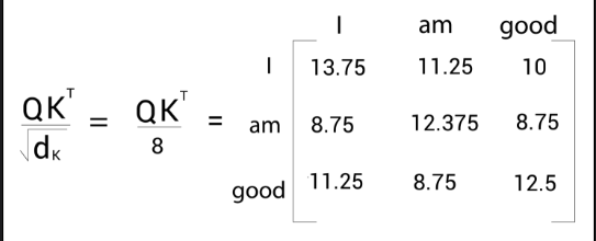
The next step in the self-attention mechanism is to divide the $Q\ast K^T$  matrix by the square root of the dimension of the key vector. But why do we have to do that? This is useful in obtaining stable gradients.

Let $d_k$ be the dimension of the key vector. Then we divide $Q\ast K^T$ by $\sqrt{d_k}$
The dimension of the key vector is 64. So, taking the square root of it, we will obtain 8. Therefore, we divide $Q\ast K^T$ by 8 as shown in the following figure:

Step 3 : Normalizing the gradients

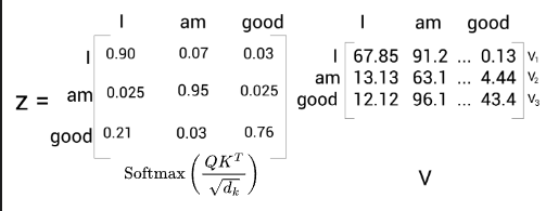
By looking at the preceding similarity scores, we can understand that they are in the unnormalized form. So, we normalize them using the softmax function. Applying the softmax function helps in bringing the score to the range of 0 to 1. The sum of the scores equals 1, as shown in the following figure:

We can call the preceding matrix a score matrix. With the help of these scores, we can understand how each word in the sentence is related to all the words in the sentence. For instance, look at the first row in the preceding score matrix. It tells us that the word ‘I’ is related to itself by 90% , to the word ‘am’ by 7%, and to the word ‘good’ by 3%.

Step 4 : Computing the attention matrix

Okay, what’s next? We computed the dot product between the query and key matrices, obtained the scores, and then normalized the scores with the softmax function. Now, the final step in the self-attention mechanism is to compute the attention matrix, 𝑍

The attention matrix contains the attention values for each word in the sentence. We can compute the attention matrix, 𝑍, by multiplying the score matrix by the value matrix $V$

$$Z=softmax\left(\frac{Q\ast K^T}{\sqrt{d_k}}\right)\ast V$$

Say we have the following:

Result of the attention matrix

Attention matrix for ‘I’

The attention matrix, 𝑍, is computed by taking the sum of the value vectors weighted by the scores. Let’s understand this by looking at it row by row. First, let’s see how for the first row, $z_1$  , the self-attention of the word ‘I’ is computed:

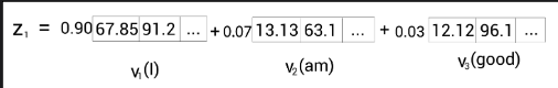
From the preceding figure, we can understand that $z_1$  , the self-attention of the word ‘I’ is computed as the sum of the value vectors weighted by the scores. Therefore, the value of  $z_1$  will contain 90% of the values from the value vector $v_1(I)$ 7% of the values from the value vector $v_2$, and 3% of values from the value vector  $v_3$,.

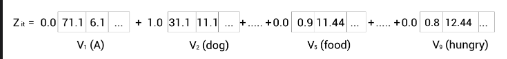
But how is this useful? To answer this question, let’s take a little detour to the example sentence we saw earlier, ‘A dog ate the food because it was hungry’. Here, the word ‘it’ indicates ‘dog’. To compute the self-attention of the word ‘it’, we follow the same preceding steps. Suppose we have the following:

Attention matrix for ‘am’

Now, coming back to our example, $z_2$ , the self-attention of the word ‘am’ is computed as the sum of the value vectors weighted by the scores, as shown in the following figure:

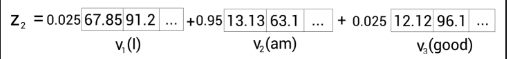
As we can observe from the preceding figure, the value of $z_2$​ will contain 2.5% of the values from the value vector $v_1$, 95% of the values from the value vector $v_2$ and 2.5% of the values from the value vector $v_3$.

Attention matrix for ‘good’

Similarly, $z_3$ , the self-attention of the word good is computed as the sum of the value vectors weighted by the scores, as shown in the following figure: 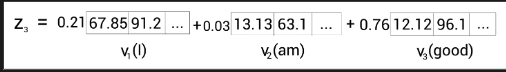his implies that the value of $z_3$ will contain 21% of the values from the value vector $v_1(I)$ 3% of the values from the value vector $v_2(am)$, and 76% of values from the value vector $v_3(good)$.

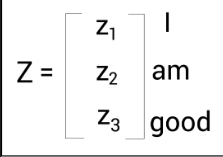
Therefore, the attention matrix, 𝑍Z, consists of self-attention values of all the words in the sentence and it is computed as follows:

$$Z=softmax\left(\frac{Q\ast K^T}{\sqrt{d_k}}\right)\ast V$$

Summary

To get a better understanding of the self-attention mechanism, the steps involved are summarized as follows:

1. We compute the dot product between the query matrix and the key matrix, $Q\ast K^T$ , and get the similarity scores.
2. We divide $Q\ast K^T$ by the square root of the dimension of the key vector $d_k$ .
3. We apply the softmax function to normalize the scores and obtain the score matrix $\frac{softmax(Q{K}^T)}{\sqrt{d_k}}$
4. We compute the attention matrix, 𝑍, by multiplying the score matrix by the value matrix 𝑉.

The self-attention mechanism is graphically shown as follows: 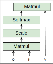The self-attention mechanism is also called scaled dot product attention, since here we are computing the dot product (between the query and key vectors) and scaling the values (with $\sqrt{d_k}$).